Ordinary Differential Equation

Ordinary Differential Equations (ODEs) are equations that relate a function to its derivatives. In simpler terms, they describe how a quantity changes with respect to another. These equations are fundamental in various fields of science and engineering, from physics and biology to economics and finance.

Key Concepts:

1. Independent Variable: The variable that the function depends on (often denoted by x or t).

2. Dependent Variable: The function itself (often denoted by y).

3. Derivative: The rate of change of the dependent variable with respect to the independent variable.

Why are ODEs important?

ODEs provide a powerful framework for modeling real-world phenomena.

They can help us understand:

• Growth and Decay: Population growth, radioactive decay, and chemical reactions.

• Motion: The movement of objects under the influence of forces (Newton’s laws of motion).

• Electrical Circuits: The flow of current and voltage in circuits.

• Heat Transfer: The distribution of heat in a material.

Types of ODEs:

• First-Order ODEs: Involve only the first derivative of the function.

• Higher-Order ODEs: Involve second, third, or higher-order derivatives.

• Linear ODEs: Have terms containing only linear combination of the function and its derivatives.

• Nonlinear ODEs: Have terms containing nonlinear combination of the function and its derivatives.

Solving ODEs:

Methods for solving ODE falls into two broad categories:

Analytical Methods:

• Separation of Variables: For certain first-order ODEs.

• Integrating Factors: For linear first-order ODEs.

• Laplace Transforms: For linear ODEs.

Numerical Methods:

For complex ODEs that cannot be solved analytically.

Visualizing Solutions:

Solutions to ODEs can often be visualized as curves or trajectories in the plane, providing insights into the behavior of the system being modeled.

First Order ODE

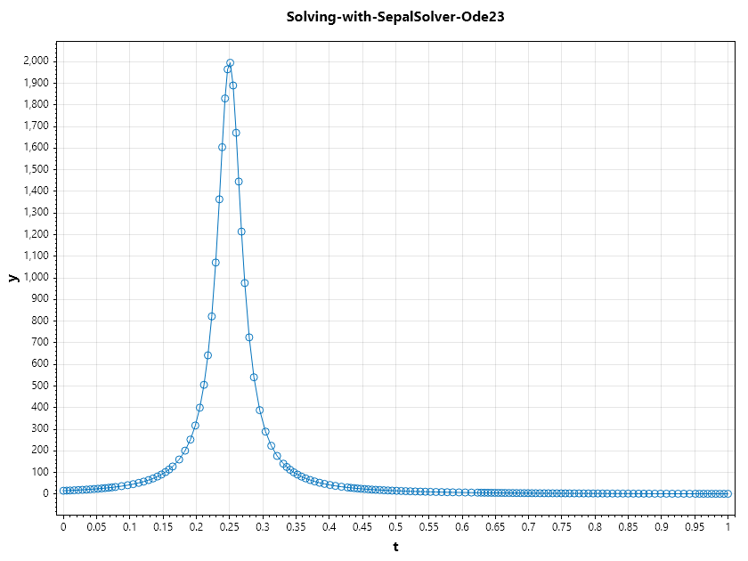
Consider: \(y' = 2(a - t)y^2\)

\[\frac{dy}{dt} = 2(a - t)y^2;\]

\[a = 0.25; y_0 = 15.9; t = [0, 1]\]

CCL-MathPythonMatlab

CCL-Math Implementation

// import libraries
using SepalSolver;
using static SepalSolver.Math;

// define the ODE
double a = 0.25;
double dydt(double t, double y) => 2 * (a - t) * y * y;

// set initial condition
double y0 = 15.9;

// set time span
double[] t_span = [0, 1];

// solve ODE
(ColVec T, Matrix Y) = Ode23(dydt, y0, t_span);

// plot the result
Plot(T, Y, "-o");
Xlabel("t"); Ylabel("y");
Title("Solving-with-CCLMath-Ode23");
SaveAs("Solving-with-CCLMath-Ode23.png");

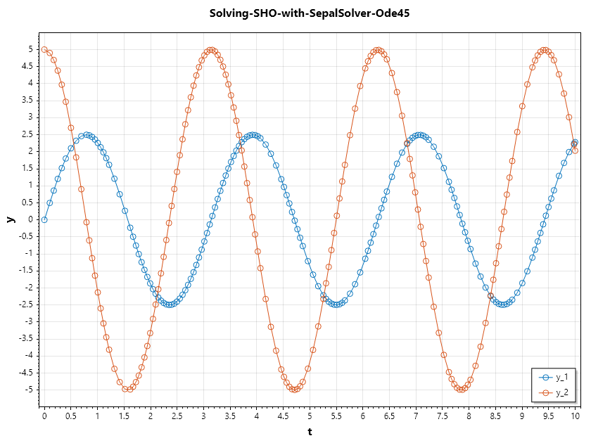
Second Order ODE

The mathematical model of a simple harmonic oscilator (SHO) results in a second order differential equation:

\[\frac{d^2y}{dt^2} = -4y\]

\[y_0 = 0; y'_0 = 5; t = [0, 10];\]

To solve this, we first transform the problem into a system of first order differential equations:

Let

\[v = \frac{dy}{dt}\]

hence

\[\frac{dv}{dt} = -4y\]

\[y_0 = 0; v_0 = 5;\]

Now we have 2 equations

\[\frac{dy}{dt} = v\]

\[\frac{dv}{dt} = -4y\]

\[y_0 = 0; v_0 = 5;\]

CCL-MathPythonMatlab

CCL-Math Implementation

// import libraries
using SepalSolver;
using static SepalSolver.Math;

// define the ODE
ColVec dzdt(double t, ColVec z)
{
   double y = z[0], v = z[1];
   double[] dz = [v, -4*y];
   return dz;
}

// set initial condition
double[] z0 = [0, 5];

// set time span
double[] t_span = [0, 10];

// solve ODE
(ColVec T, Matrix Y) = Ode45(dzdt, z0, t_span);

// plot the result
Plot(T, Y, "-o");
Xlabel("t"); Ylabel("y");
Title("Solving-SHO-with-CCLMath-Ode45");
Legend = (["y_1", "y_2"], Alignment.LowerRight");
SaveFig("Solving-SHO-with-CCLMath-Ode45.png");