Generates a histogram representation of a data vector.
This method bins the input values into intervals and returns the histogram data,
including counts per bin, positions (typically bin centers), bin size, and min/max of the data range.
Suitable for visualizing data distributions.
Generates coordinate matrices from coordinate vectors.
This method creates two 2D arrays representing all pairs of x and y coordinates from the input vectors, which is often used for evaluating functions over a grid.
Reads a two-dimensional elements in matrix from a file.
This method loads space-separated integers from each line of the specified file and constructs a matrix representation.
MatrixReadMatrix(stringfilename)
Parameters:
filename:
The path to the input file containing the matrix data.
Returns:
A two-dimensional integer array containing the values read from the file.
Reads a row vector of numbers from a file.
This method parses a single line of space-separated values from the specified file and constructs a one-dimensional matrix representation.
RowVecReadRowVec(stringfilename)
Parameters:
filename:
The path to the input file containing the row vector data.
Returns:
A one-dimensional matrix representing the row vector read from the file.
Reads a column vector of numbers from a file.
This method parses multiple lines of input from the specified file, with each line representing a single value in the column vector.
ColVecReadColVec(stringfilename)
Parameters:
filename:
The path to the input file containing the column vector data.
Returns:
A one-dimensional matrix representing the column vector read from the file.
Example:
Read a column vector from a file named “colvec.txt”:
Writes a two-dimensional matrix of integers to a file.
This method serializes the matrix in space-separated format, with each row written on a new line in the target file.
voidWriteMatrix(MatrixA,stringfilename)
Parameters:
A:
The matrix object to be written to the file.
filename:
The path to the output file where the matrix will be saved.
Returns:
This method does not return a value (being a void method)
Example:
Write a matrix to a file named “matrixA.txt”:
// import librariesusingSystem;usingstaticSepalSolver.Math;stringpath="matrixA.txt";// Create a matrixMatrixA=newdouble[,]{{12,18,3},{15,25,30}};// Write to fileWriteMatrix(A,path);
Determines whether all values in a one-dimensional or two-dimensional array are true.
This method checks each element in the input array and returns true only if all values are true; otherwise, false.
boolAll(bool[]A)boolAll(bool[,]A)
Parameters:
A:
The array of Boolean values to evaluate.
Returns:
True, if all elements in the array are true; otherwise, false.
Example:
Check if all values in a Boolean array or matrix are true:
Determines whether any value in a one-dimensional or two-dimensional array is true.
This method checks each element in the input array and returns true if at least one value is true; otherwise, false.
boolAny(bool[]A)boolAny(bool[,]A)
Parameters:
A:
The array of Boolean values to evaluate.
Returns:
True, if at least one element in the array is true; otherwise, false.
Returns the indices of true values in a Boolean array or matrix, up to a maximum of k matches.
This method scans the input array and collects the positions of all values that evaluate to true, up to the specified limit.
Computes the quotient and remainder of integer division.
This method performs an integer division of a dividend, a by a divisor, b and returns both the quotient and remainder as a tuple.
(int,int)DivRem(inta,intb)
Parameters:
a:
The dividend—value to be divided.
b:
The divisor—value by which to divide.
Returns:
A tuple containing the integer quotient and remainder:(quotient, remainder).
Example:
Divide 17 by 5 and get both the quotient and remainder:
Converts a double-precision floating-point number to its string representation.
This method transforms the numeric input into a human-readable string format, suitable for display or formatting purposes.
Applies a scalar function to each element of a column vector or row vector or matrix.
This method maps a user-defined function across every element in the input array or matrix and produces a transformed array or matrix of the same size.
Reshapes a one-dimensional array of input into a matrix with specified dimensions.
This method returns a output with the given dimensions, populated with the data from the input array.
Calculates the length of the hypotenuse of a right-angled triangle given the lengths of the other two sides.This method computes z = Sqrt(Pow(x, 2) + Pow(y, 2)) by avoiding underflow and overflow.
Calculates the absolute value of an input.
This method returns the absolute value of the given input, which is the non-negative value of the input without regard to its sign.
Generates a one-dimensional 0r two-dimensional array of zeros with specified dimensions.
This method creates a vector of M rows or matrix of M rows and N columns, where every element is initialized to zero.
Generates a two-dimensional array of ones with specified dimensions.
This method creates a matrix of M rows and N columns, where every element is initialized to 1.0.
Array of integer rows and columns in the resulting matrix.
Returns:
An array of vector of size M or matrix of size M by N filled with ones.
Example:
Create a 2x3 matrix of ones:
// import librariesusingSystem;usingstaticSepalSolver.Math;//Generate Matrix 2 by 3 with all the element has 1.0Matrixones=Ones(2,3);// Display matrixConsole.WriteLine(ones);
Replicates a scalar value across a one-dimensional array or two-dimensional matrix of specified size.
This method returns a vector of size M or matrix of size M x N in which every element is initialized to the scalar value <c>A</c>.
Array of integer rows and columns in the resulting matrix.
Returns:
A matrix of dimensions M x N where all values are equal to A.
Example:
Create a 2x4 matrix filled with the value 3.14:
// import librariesusingSystem;usingstaticSepalSolver.Math;// Replicate all elements of a matrix same.Matrixreplicated=Repmat(pi,2,4);// Display matrixConsole.WriteLine(replicated);
Replicates each element of a matrix a specified number of times along both axes.
This method expands the input matrix by repeating each element M times row-wise (vertically) and N times column-wise (horizontally), returning the result as a new Matrix with repetitive elements.
MatrixRepelem(MatrixA,intM,intN)
Parameters:
A:
The input matrix whose elements will be replicated.
M:
The number of times to repeat each element along the row (vertical) direction.
N:
The number of times to repeat each element along the column (horizontal) direction.
Returns:
A new Matrix instance containing the expanded result with replicated elements.
Example:
Create a 4x6 matrix by replicating a 2x2 matrix:
// import librariesusingSystem;usingstaticSepalSolver.Math;// Create a 2 by 2 matrixMatrixA=newdouble[,]{{1,2},{3,4}};// Apply element-wise replicationMatrixexpanded=Repelem(A,2,3);// Display resultConsole.WriteLine(expanded);
Computes the Kronecker product of two matrices.
This method generates a block matrix by multiplying each element of matrix X by the entire matrix Y, preserving the structure of X.
MatrixKron(MatrixX,MatrixY)
Parameters:
X:
The first matrix (left operand) of the Kronecker product.
Y:
The second matrix (right operand) of the Kronecker product.
Returns:
A Matrix representing the Kronecker product of X and Y.
Example:
Compute the Kronecker product of two 2x2 matrices:
// import librariesusingSystem;usingstaticSepalSolver.Math;// create a 2 by 2 matrixMatrixA=newdouble[,]{{1,2},{3,4}};;// create a 2 by 2 matrixMatrixB=newdouble[,]{{0,5},{6,7}};// Compute Kronecker productMatrixresult=Kron(A,B);// Display resultConsole.WriteLine(result);
Generates a one-dimensional or two-dimensional matrix of random double-precision values between 0.0 (inclusive) and 1.0 (exclusive).
This method creates a matrix with M rows and N columns, where each element is independently sampled from a uniform distribution.
Generates an array (Vector) or matrix of normally distributed random double values.
This method creates a vector of size M or M * N matrix with each element independently sampled from a normal distribution characterized by the specified <c>mean</c> and <c>standard deviation</c>.
Generates a matrix of random double values from a triangular distribution.
This method creates an M x N matrix where each element is independently sampled from a triangular distribution defined by minimum bound value, mode of distribution likely, and maximum bound value.
Generates a linearly spaced array of double values between two endpoints.
This method produces a one-dimensional array of N evenly spaced values from a to b, inclusive. If N is 1, the array contains just a.
double[]Linspace(doublea,doubleb,intN=100)
Parameters:
a:
The starting value of the range.
b:
The ending value of the range.
N:
The number of evenly spaced points to generate. Default is 100.
Returns:
An array containing N linearly spaced values between a and b.
Example:
Generate 10 points from -1 to 1:
// import librariesusingSystem;usingstaticSepalSolver.Math;//Generate point from -1 to 1RowVecline=Linspace(-1.0,1.0,10);// Display resultConsole.WriteLine(line);
Generates a logarithmically spaced array of double values between powers of 10.
This method creates a one-dimensional array with N values spaced evenly on a logarithmic scale, ranging from <c>10^a</c> to <c>10^b</c>, inclusive.
double[]Logspace(doublea,doubleb,intN=100)
Parameters:
a:
The base-10 exponent of the starting value (10^a).
b:
The base-10 exponent of the ending value (10^b).
N:
The number of points to generate. Default is 100.
Returns:
An array of N values logarithmically spaced between 10^a and 10^b.
Example:
Generate 5 values from 10⁰ to 10²:
// import librariesusingSystem;usingstaticSepalSolver.Math;// Generate logarithmically space between 1 and 100 inclusiveRowVecfreqs=Logspace(0,2,5);// Display result,Console.WriteLine(freqs);
Performs one-dimensional linear interpolation.
This method estimates the output value at a query point <c>x</c> by linearly interpolating between known data points in <c>X</c> and corresponding values in <c>Y</c>.
// import librariesusingSystem;usingstaticSepalSolver.Math;ColVecX=newColVec(newdouble[]{0.0,1.0,2.0,3.0});ColVecY=newColVec(newdouble[]{0.0,10.0,20.0,30.0});doublex=1.5;doubley=Interp1(X,Y,x);Console.WriteLine($"Interpolated value at x=1.5: {y}");
Extracts a specified column from a two-dimensional array.
This method retrieves the column at index j from the input matrix data and returns it as a one-dimensional array.
double[]Getcol(intj,double[,]data)
Parameters:
j:
The zero-based index of the column to extract.
data:
The two-dimensional array from which the column will be retrieved.
Returns:
An array representing the j_th column of the matrix data.
Example:
Extract the first column from a 3x3 matrix:
// import librariesusingSystem;usingstaticSepalSolver.Math;// Create 3 by 3 matrixdouble[,]matrix=newdouble[,]{{1.0,2.0,3.0},{4.0,5.0,6.0},{7.0,8.0,9.0}};// Get column 0 (first column)ColVeccol=Getcol(0,matrix);// DisplayConsole.WriteLine(col);
Extracts a specified row from a two-dimensional array.
This method retrieves the row at index i from the input matrix data and returns it as a one-dimensional array.
double[]Getrow(inti,double[,]data)
Parameters:
i:
The index of the row to extract.
data:
The two-dimensional array from which the row will be retrieved.
Returns:
An array representing the i-th row of matrix data element.
Example:
Extract the third row from a 4x3 matrix:
// import librariesusingSystem;usingstaticSepalSolver.Math;// Create a 4 by 3 matrixdouble[,]matrix={{1.0,2.0,3.0},{4.0,5.0,6.0},{7.0,8.0,9.0},{10.0,11.0,12.0}};// Get row 2 (third row)RowVecrow=Getrow(2,matrix);// Output the matrixConsole.WriteLine(row);
Extracts specified columns from a two-dimensional array using an indexer.
This method returns a new Matrix containing only the columns of data specified by the I-indexer.
MatrixGetcols(indexerI,double[,]data)
Parameters:
I:
An indexer object specifying the zero-based column indices to select.
data:
The two-dimensional array from which columns are extracted.
Returns:
A Matrix composed of the selected columns from the input matrix data, in the order defined by I-indexer.
Example:
Extract columns 1 and 3 from a 3x4 matrix:
// import librariesusingSystem;usingstaticSepalSolver.Math;// Create a 3 by 4 matrixdouble[,]matrix=newdouble[,]{{10,20,30,40},{50,60,70,80},{90,100,110,120}};// Extract the 2nd and 4th columnsMatrixcols=Getcols([1,3],matrix);// Output the extracted matrixConsole.WriteLine(cols);
Extracts specified rows from a two-dimensional array using an indexer.
This method returns a new Matrix data composed of the rows from matrix data that correspond to the indices specified by I-indexer.
MatrixGetrows(indexerI,double[,]data)
Parameters:
I:
An indexer object that specifies the zero-based indices of the rows to extract.
data:
The two-dimensional array from which rows will be selected.
Returns:
A Matrix containing the rows of data specified by I-indexer, in the same order.
Example:
Extract the 1st and 3rd rows from a 4x3 matrix:
// import librariesusingSystem;usingstaticSepalSolver.Math;// Create a 4 by 3 matrixdouble[,]matrix=newdouble[,]{{10,20,30,40},{50,60,70,80},{90,100,110,120}};// Extract the first and third rowsMatrixrows=Getrows([0,2],matrix);// Output the extracted matrixConsole.WriteLine(rows);
Horizontally concatenates a scalar with a row vector. Also concatenates a matrix with a matrix. The two matrices must have equal row count.
This method concatenate a scalar value to a vector or matrix to a matrix and other combination returning a new vector or matrix with an additional leading element.
The input array (row or column vector) or matrix to which a will be prepended.
Returns:
A vector or matrix consisting of concatenated values.
Example:
Concatenate the value 1.0 to a row vector:
// import librariesusingSystem;usingstaticSepalSolver.Math;// Create a row vectorRowVecB=newRowVec(newdouble[]{2.0,3.0,4.0});// Concatenate the scaler value and the vector together.RowVecresult=Hcart(1.0,B);// Output the resultconsole.writeline($"The concatenated matrix is: {rows}")
Output:
1
2
3
4
Example:
Horizontally concatenate two 2x2 matrices:
// import librariesusingSystem;usingstaticSepalSolver.Math;// Create a 2 by 2 matrixMatrixA=newdouble[,]{{1,2},{3,4}};// Create a 2 by 2 matrixMatrixB=newdouble[,]{{5,6},{7,8}};ConcatenatethetwomatrixtogetherMatrixresult=Hcart(A,B);// Output the resultconsole.writeline($"The concatenated matrix is: {result}")
Vertically concatenates a scalar with a column vector or concatenates a matrix with a matrix. The two matrices must equal column count.
concatenate a scalar value to a vector or matrix to a matrix and other combination returning a new vector or matrix with an additional leading element.
The scalar value to be placed at the top or below of the resulting vector.
A, B:
The input column vector or matrix whose elements will appear before or after a.
Returns:
A vector or matrix consisting of a followed by the entries of B.
Example:
Prepend a scalar to a column vector:
// import librariesusingSystem;usingstaticSepalSolver.Math;// Create a vectorColVecB=newdouble[]{2.0,3.0,4.0};// Concatenate the scalar value and the vector togetherColVecresult=Vcart(1.0,B);// Output the resultconsole.writeline($"The concatenated matrix is: {result}")
Output:
1
2
3
4
Example:
Vertically concatenate two 2x2 matrices:
// import librariesusingSystem;usingstaticSepalSolver.Math;// Create 2 by 2 matrixMatrixA=newMatrix(newdouble[,]{{1,2},{3,4}});// Create 2 by 2 matrixMatrixB=newMatrix(newdouble[,]{{5,6},{7,8}});//Concatenate the two matricesMatrixresult=Vcart(A,B);// Output the resultconsole.writeline($"The concatenated matrix is: {result}")
Raises a real or complex numbers or elements in a vector or matrix to the power of another.
This method computes the result of raising x to the power n, returning x^n.
Computes the first-order discrete difference of a one-dimensional or two-dimensional array.
This method returns a new array where each element is the difference between consecutive elements of the input array X.
Rounds a floating-point number or complex number or each element in a vector or matrix to a specified number of decimal places.
This method returns a double value rounded to the nearest number with the specified number of decimal places using standard rounding rules (round half to even).
The double-precision floating-point number or complex number or each element in a vector or matrix to be rounded.
decP:
The number of decimal places to round to. Default is 0 (rounds to nearest integer). Must be between 0 and 15.
Returns:
A double value rounded to the specified number of decimal places.
Example:
Round a number, 3.14159 to the nearest integer:
// import librariesusingSystem;usingstaticSepalSolver.Math;// Create a double valuedoublevalue=3.14159;// Round to nearest integer (default behavior)doubleresult=Round(value,0);// Output the resultconsole.writeline($"The rounded value is: {result}")
Calculates the square root of a specified number.
This method returns the positive square root of the input value. For negative inputs, the result is NaN (Not a Number).
The number whose square root is to be calculated. Must be non-negative for real results.
Returns:
The positive square root of x. Returns NaN if x is negative, and positive infinity if x is positive infinity.
Example:
Calculate the square root of a positive number, 25:
// import librariesusingSystem;usingstaticSepalSolver.Math;// Create a double valuedoublevalue=25.0;// Calculate the square rootdoubleresult=Sqrt(value);// Output the resultconsole.writeline($"The square root is: {result}")
The square of x (x * x). Returns positive infinity if the result overflows.
Example:
Calculate the square of a positive number:
// import librariesusingSystem;usingstaticSepalSolver.Math;// Create a double valuedoublevalue=5.0;// Calculate the squaredoubleresult=Sqr(value);// Output the resultconsole.writeline($"The square is: {result}")
Returns the largest integer less than or equal to the specified number.
This method rounds down to the nearest integer, always moving toward negative infinity regardless of the sign of the input.
doubleFloor(doublex)
Parameters:
x:
The double-precision floating-point number to floor.
Returns:
The largest integer less than or equal to x. If x is already an integer, returns x unchanged.
Example:
Floor a positive decimal number:
// import librariesusingSystem;usingstaticSepalSolver.Math;// Create a positive decimal valuedoublevalue=4.7;// Calculate the floordoubleresult=Floor(value);// Output the resultconsole.writeline($"The floor is: {result}")
Returns the smallest integer greater than or equal to the specified number.
This method rounds up to the nearest integer, always moving toward positive infinity regardless of the sign of the input.
doubleCeil(doublex)
Parameters:
x:
The double-precision floating-point number to ceiling.
Returns:
The smallest integer greater than or equal to x. If x is already an integer, returns x unchanged.
Example:
Ceiling a positive decimal number:
// import librariesusingSystem;usingstaticSepalSolver.Math;// Create a positive decimal valuedoublevalue=4.2;// Calculate the ceilingdoubleresult=Ceil(value);// Output the resultconsole.writeline($"The ceiling is: {result}")
Returns the larger of two or more real or, floating-point number or maximum among elelments of a vector or matrices.
This method compares two integer values and returns the one with the greater value.
The maximum number from two or more given vectors or matrices. If A and B are equal, returns either value.
Example:
Find the maximum of two positive integers:
// import librariesusingSystem;usingstaticSepalSolver.Math;// Create two integer valuesintvalueA=15;intvalueB=23;// Find the maximumintresult=Max(valueA,valueB);// Output the resultconsole.writeline($"The maximum is: {result}")
Output:
23
Example:
Find the element-wise maximum of two 2x2 matrices:
// import librariesusingSystem;usingstaticSepalSolver.Math;// Create first 2x2 matrixMatrixA=newMatrix(newdouble[,]{{1,8},{5,2}});// Create second 2x2 matrixMatrixB=newMatrix(newdouble[,]{{3,4},{1,7}});// Find element-wise maximumMatrixresult=Max(A,B);// Output the resultconsole.writeline($"The maximum is: {result}")
The smaller of the two input values. If A and B are equal, returns either value.
Example:
Find the minimum of two positive integers:
// import librariesusingSystem;usingstaticSepalSolver.Math;// Create two integer valuesintvalueA=15;intvalueB=23;// Find the minimumintresult=Min(valueA,valueB);// Output the resultconsole.writeline($"The minimum is: {result}")
Calculates the sine of the specified angle in radians.
This method returns the sine of the input angle, where the angle is measured in radians. The result is between -1 and 1.
The angle in radians for which to calculate the sine.
Returns:
The sine of x, ranging from -1 to 1. Returns 0 if x is positive or negative infinity.
Example:
Calculate the sine of common angles:
// import librariesusingSystem;usingstaticSepalSolver.Math;// Calculate sine of π/2 radians (90 degrees)doubleangle=Pi/2;doubleresult=Sin(angle);// Output the resultconsole.writeline($"Sin(π/2) = {result}")
Calculates the arcsine (inverse sine) of the specified value.
This method returns the angle in radians whose sine is the specified value. The input must be between -1 and 1, and the result is between -π/2 and π/2.
The sine value for which to calculate the arcsine. Must be between -1 and 1 inclusive.
Returns:
The angle in radians whose sine equals x, ranging from -π/2 to π/2. Returns NaN if x is outside the range [-1, 1].
Example:
Calculate the arcsine of common values:
// import librariesusingSystem;usingstaticSepalSolver.Math;// Calculate arcsine of 1 (which should be π/2)doublevalue=1.0;doubleresult=Asin(value);// Output the resultconsole.writeline($"Asin(1) = {result}")
Output:
Asin(1) = 1.5707963267948966
Example:
Calculate the arcsine of zero and negative values:
// import librariesusingSystem;usingstaticSepalSolver.Math;// Calculate arcsine of 0 and -1doubleasinZero=Asin(0);doubleasinNegativeOne=Asin(-1);// Output the resultsconsole.writeline($"Asin(0) = {asinZero}")console.writeline($"Asin(-1) = {asinNegativeOne}")
Calculates the cosine of the specified angle in radians.
This method returns the cosine of the input angle, where the angle is measured in radians. The result is between -1 and 1.
Calculates the arccosine (inverse cosine) of the specified value.
This method returns the angle in radians whose cosine is the specified value. The input must be between -1 and 1, and the result is between 0 and π.
A scalar number or one-dimensional or two-dimensional array for which to calculate the arccosine. Must be between -1 and 1 inclusive.
Returns:
The angle in radians whose cosine equals x, ranging from 0 to π. Returns NaN if x is outside the range [-1, 1].
Example:
Calculate the arccosine of common values:
// import librariesusingSystem;usingstaticSepalSolver.Math;// Calculate arccosine of 1 (which should be 0)doublevalue=1.0;doubleresult=Acos(value);// Output the resultconsole.writeline($"Acos(1) = {result}")
Calculates the tangent of the specified angle in radians.
This method returns the tangent of the input angle, where the angle is measured in radians. The tangent function has vertical asymptotes at odd multiples of π/2.
Computes the arctangent (inverse tangent) of a specified number.
This method returns the angle in radians whose tangent is the specified number. The angle is in the range -π/2 to π/2 radians.
Computes the hyperbolic sine of a specified number.
This method returns the hyperbolic sine of x, defined as (e^x - e^(-x))/2. The hyperbolic sine function is an odd function with domain (-∞, +∞) and range (-∞, +∞).
A scalar number one-dimensional or two-dimensional array representing the value for which the hyperbolic sine is to be computed.
Returns:
A double representing the hyperbolic sine of x.
Returns PositiveInfinity if x is PositiveInfinity.
Returns NegativeInfinity if x is NegativeInfinity.
Returns NaN if x is NaN.
Example:
Calculate the hyperbolic sine of a positive value:
// Import librariesusingSystem;usingstaticSepalSolver.Math;// Define the input valuedoublex=2.0;// Calculate the hyperbolic sinedoubleresult=Sinh(x);// Output the resultConsole.WriteLine($"Sinh({x}) = {result}");Console.WriteLine($"Verification: (e^{x} - e^(-{x}))/2 = {(Exp(x) - Exp(-x)) / 2}");
Computes the hyperbolic cosine of a specified number.
This method returns the hyperbolic cosine of x, defined as (e^x + e^(-x))/2. The hyperbolic cosine function is an even function with domain (-∞, +∞) and range [1, +∞).
A scalar number or one-dimensional or two-dimensional array representing the value for which the hyperbolic cosine is to be computed.
Returns:
A double representing the hyperbolic cosine of x, always greater than or equal to 1.
Returns PositiveInfinity if x is PositiveInfinity or NegativeInfinity.
Example:
Calculate the hyperbolic cosine of a positive value:
// Import librariesusingSystem;usingstaticSepalSolver.Math;// Define the input valuedoublex=1.5;// Calculate the hyperbolic cosinedoubleresult=Cosh(x);// Output the resultConsole.WriteLine($"Cosh({x}) = {result}");Console.WriteLine($"Verification: (e^{x} + e^(-{x}))/2 = {(Math.Exp(x) + Math.Exp(-x)) / 2}");
Computes the hyperbolic tangent of a given value.
The hyperbolic tangent is defined as (e^x - e^(-x)) / (e^x + e^(-x)) and maps any real number to the range (-1, 1).
A double-precision floating-point number representing the value for which to calculate the hyperbolic tangent.
Returns:
The hyperbolic tangent of a number.
Example:
Evaluate hyperbolic tangent of the number, 1
// import librariesusingSystem;usingstaticSepalSolver.Math;// Compute the hyperbolic tangent of a numberdoubleresult=Tanh(1.0);// Output the resultConsole.WriteLine($"Tanh(1.0) = {result}");
Calculates the inverse hyperbolic tangent (area hyperbolic tangent) of a specified value.
The inverse hyperbolic tangent is defined as 0.5 * ln((1 + x) / (1 - x)).
The function is undefined for values less than or equal to -1 and greater than or equal to 1.
A one-dimensional or two-dimensional array or double-precision floating-point number in the range (-1, 1), representing the value for which to compute the inverse hyperbolic tangent.
Returns:
The inverse hyperbolic tangent of the number, x.
Example:
Evaluate the inverse hyperbolic tangent of the number, 0.5.
// import librariesusingSystem;usingstaticSepalSolver.Math;// Compute the inverse hyperbolic tangent of a numberdoubleresult=Atanh(0.5);// Output the resultConsole.WriteLine($"Atanh(0.5) = {result}");
A one-dimensional or two-dimensional array or double-precision floating-point number representing the power to raise Euler’s number (e) to.
Returns:
The exponential of a number, i.e., e raised to the power x.
Example:
Evaluate the exponential value of number, 2.
// import librariesusingSystem;usingstaticSepalSolver.Math;// Compute the exponential of a numberdoubleresult=Exp(2.0);// Output the resultConsole.WriteLine($"Exp(2.0) = {result}");
A one-dimensional or two-dimensional array or double-precision floating-point number greater than zero, representing the value whose logarithm is to be calculated.
Returns:
The natural logarithm (ln) of a number.
Example:
Evaluate the natural logaraithm of the number, 10
// import librariesusingSystem;usingstaticSepalSolver.Math;// Compute the natural logarithm of a numberdoubleresult=Log(10.0);// Output the resultConsole.WriteLine($"Log(10.0) = {result}");
A one-dimensional or two-dimensional array or double-precision floating-point number greater than zero, representing the value whose base-2 logarithm is to be calculated.
Returns:
The base-2 logarithm of the number, x.
Example:
Evaluate log 16 to base 2.
// import librariesusingSystem;usingstaticSepalSolver.Math;// Compute the base-2 logarithm of a numberdoubleresult=Log2(16.0);// Output the resultConsole.WriteLine($"Log2(16.0) = {result}");
A one-dimensional or two-dimensional array or double-precision floating-point number greater than zero, representing the value whose base-10 logarithm is to be calculated.
Returns:
The base-10 logarithm (common logarithm) of the number, x.
Example:
Evaluate the logarithm of 1000 to base 10.
// import librariesusingSystem;usingstaticSepalSolver.Math;// Compute the base-10 logarithm of a numberdoubleresult=Log10(1000.0);// Output the resultConsole.WriteLine($"Log10(1000.0) = {result}");
Computes the modified Bessel function of the first kind Iₙ(x).
This method evaluates the exponentially scaled modified Bessel function of the first kind for a given order and value.
Computes the Bessel function of the second kind Yₙ(x).
This method evaluates the Weber or Neumann Bessel function of the first kind for a given order and value.
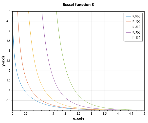
Computes the Modified Bessel function of the second kind Kₙ(x).
This method evaluates the exponentially scaled modified Bessel function for a given order and value.
Computes the Chebyshev polynomial of the first kind of degree n evaluated at x.
This method returns the value of the nth Chebyshev polynomial T_n(x) at the specified point. Chebyshev polynomials of the first kind are defined by:
.math: ‘T_n(cos(θ)) = cos(nθ)’ and satisfy the recurrence relation:
.math: ‘T_0(x) = 1,’
.math: ‘T_1(x) = x,’
.math: ‘T_n(x) = 2xT_{n-1}(x) - T_{n-2}(x)’
The degree of the Chebyshev polynomial. Must be a non-negative integer.
x:
The single point or points within array or matrix at which to evaluate the Chebyshev polynomial. Typically in the range [-1, 1] for optimal numerical properties.
Returns:
A scalar point of point in an array for matrix form representing the value of the nth Chebyshev polynomial of the first kind evaluated at x.
Returns NaN if n is negative or if computation fails.
Example:
Calculate the first few Chebyshev polynomials at x = 0.5:
// Import librariesusingSystem;usingstaticSepalSolver.Math;// Define the evaluation pointdoublex=0.5;// Calculate the first few Chebyshev polynomialsdoubleT0=ChebyshevT(0,x);// T_0(x) = 1doubleT1=ChebyshevT(1,x);// T_1(x) = xdoubleT2=ChebyshevT(2,x);// T_2(x) = 2x² - 1doubleT3=ChebyshevT(3,x);// T_3(x) = 4x³ - 3x// Output the resultsConsole.WriteLine($"Chebyshev polynomials evaluated at x = {x}:");Console.WriteLine($"T_0({x}) = {T0}");Console.WriteLine($"T_1({x}) = {T1}");Console.WriteLine($"T_2({x}) = {T2}");Console.WriteLine($"T_3({x}) = {T3}");
Output:
Chebyshev polynomials evaluated at x = 0.5:
T_0(0.5) = 1
T_1(0.5) = 0.5
T_2(0.5) = -0.5
T_3(0.5) = -1
Computes the Chebyshev polynomial of the second kind of degree n evaluated at x.
This method returns the value of the nth Chebyshev polynomial U_n(x) at the specified point.
Chebyshev polynomials of the second kind are defined by U_n(cos(θ)) = sin((n+1)θ)/sin(θ) and
satisfy the recurrence relation U_0(x) = 1, U_1(x) = 2x, U_n(x) = 2xU_{n-1}(x) - U_{n-2}(x).
The degree of the Chebyshev polynomial of the second kind. Must be a non-negative integer.
x:
The point at which to evaluate the Chebyshev polynomial. Typically in the range [-1, 1] for optimal numerical properties.
Returns:
A Scaler point or points in an array or matrix form representing the value of the nth Chebyshev polynomial of the second kind evaluated at x.
Returns NaN if n is negative or if computation fails.
Example:
Calculate the first few Chebyshev polynomials of the second kind at x = 0.5:
// Import librariesusingSystem;usingstaticSepalSolver.Math;// Define the evaluation pointdoublex=0.5;// Calculate the first few Chebyshev polynomials of the second kinddoubleU0=ChebyshevU(0,x);// U_0(x) = 1doubleU1=ChebyshevU(1,x);// U_1(x) = 2xdoubleU2=ChebyshevU(2,x);// U_2(x) = 4x² - 1doubleU3=ChebyshevU(3,x);// U_3(x) = 8x³ - 4x// Output the resultsConsole.WriteLine($"Chebyshev polynomials of the second kind at x = {x}:");Console.WriteLine($"U_0({x}) = {U0}");Console.WriteLine($"U_1({x}) = {U1}");Console.WriteLine($"U_2({x}) = {U2}");Console.WriteLine($"U_3({x}) = {U3}");
Output:
Chebyshev polynomials of the second kind at x = 0.5:
U_0(0.5) = 1
U_1(0.5) = 1
U_2(0.5) = 0
U_3(0.5) = -1
Computes the Legendre polynomial of degree n evaluated at x.
This method returns the value of the nth Legendre polynomial P_n(x) at the specified point. Legendre polynomials are orthogonal polynomials on the interval [-1, 1] that satisfy the recurrence relation P_0(x) = 1, P_1(x) = x, and (n+1)P_{n+1}(x) = (2n+1)xP_n(x) - nP_{n-1}(x). They are solutions to Legendre’s differential equation.
The degree of the Legendre polynomial. Must be a non-negative integer.
x:
The point at which to evaluate the Legendre polynomial. Can be any real number, but orthogonality properties hold on [-1, 1].
Returns:
A scalar point or points in an array or matrix form representing the value of the nth Legendre polynomial evaluated at x.
Returns NaN if n is negative or if computation fails.
Example:
Calculate the first few Legendre polynomials at x = 0.5:
// Import librariesusingSystem;usingstaticSepalSolver.Math;// Define the evaluation pointdoublex=0.5;// Calculate the first few Legendre polynomialsdoubleP0=LegendreP(0,x);// P_0(x) = 1doubleP1=LegendreP(1,x);// P_1(x) = xdoubleP2=LegendreP(2,x);// P_2(x) = (3x² - 1)/2doubleP3=LegendreP(3,x);// P_3(x) = (5x³ - 3x)/2doubleP4=LegendreP(4,x);// P_4(x) = (35x⁴ - 30x² + 3)/8// Output the resultsConsole.WriteLine($"Legendre polynomials evaluated at x = {x}:");Console.WriteLine($"P_0({x}) = {P0}");Console.WriteLine($"P_1({x}) = {P1}");Console.WriteLine($"P_2({x}) = {P2}");Console.WriteLine($"P_3({x}) = {P3}");Console.WriteLine($"P_4({x}) = {P4}");
Computes the Legendre function of the second kind (also known as Legendre Q function) of degree n at point x.
The Legendre Q function is the second linearly independent solution to Legendre’s differential equation and is used in engineering applications involving spherical coordinates and potential theory.
The degree (order) of the Legendre Q function. Must be a non-negative integer (n >= 0).
x:
The argument at which to evaluate the Legendre Q function. Must satisfy |x| > 1 for real-valued results, as the function has singularities at x = ±1.
Returns:
The value of the Legendre Q function of degree n evaluated at x. Returns a double-precision floating-point number or one-dimensional or two-dimensional array.
Example:
Compute the Legendre Q function of degree 0 at x = 2.0:
// import librariesusingSystem;usingstaticSepalSolver.Math;// Define the degree and argumentintn=0;doublex=2.0;// Calculate the Legendre Q functiondoubleresult=LegendreQ(n,x);// Output the resultConsole.WriteLine($"Q_0(2.0) = {result});
Output:
Q_0(2.0) = 0.549306
Example:
Compute the Legendre Q function of degree 2 at x = 1.5:
// import librariesusingSystem;usingstaticSepalSolver.Math;// Define the degree and argumentintn=2;doublex=1.5;// Calculate the Legendre Q functiondoubleresult=LegendreQ(n,x);// Output the resultConsole.WriteLine($"Q_2(1.5) = {result});
Output:
Q_2(1.5) = -0.581633
Example:
Compare Legendre Q functions of different degrees at x = 3.0:
// import librariesusingSystem;usingstaticSepalSolver.Math;// Define the argumentdoublex=3.0;// Calculate Legendre Q functions for degrees 0, 1, and 2doubleq0=LegendreQ(0,x);doubleq1=LegendreQ(1,x);doubleq2=LegendreQ(2,x);// Output the resultsConsole.WriteLine($"Q_0(3.0) = {q0}");Console.WriteLine($"Q_1(3.0) = {q1}");Console.WriteLine($"Q_2(3.0) = {q2}");
Computes the Hermite polynomial H_n(x) of degree n at point x using the physicists’ convention.
The Hermite polynomials are orthogonal polynomials that arise in quantum mechanics (harmonic oscillator wavefunctions), probability theory (Gaussian integrals), and numerical analysis. They satisfy the recurrence relation H_{n+1}(x) = 2xH_n(x) - 2nH_{n-1}(x).
The degree (order) of the Hermite polynomial. Must be a non-negative integer (n >= 0).
x:
The argument at which to evaluate the Hermite polynomial. Can be any real scalar number or numbers in array or matrix form.
Returns:
The value of the Hermite polynomial H_n(x) evaluated at x. Returns a double-precision floating-point number or one dimensional or two dimensional array.
Example:
Compute the Hermite polynomial of degree 0 at x = 1.0:
// import librariesusingSystem;usingstaticSepalSolver.Math;// Define the degree and argumentintn=0;doublex=1.0;// Calculate the Hermite polynomialdoubleresult=HermiteH(n,x);// Output the resultConsole.WriteLine($"H_0(1.0) = {result}");
Output:
H_0(1.0) = 1.000000
Example:
Compute the Hermite polynomial of degree 3 at x = 2.0:
// import librariesusingSystem;usingstaticSepalSolver.Math;// Define the degree and argumentintn=3;doublex=2.0;// Calculate the Hermite polynomialdoubleresult=HermiteH(n,x);// Output the resultConsole.WriteLine($"H_3(2.0) = {result}");
Computes the Laguerre polynomial L_n(x) of degree n at point x.
The Laguerre polynomials are orthogonal polynomials that arise in quantum mechanics (hydrogen atom wavefunctions), mathematical physics, and numerical analysis. They satisfy the recurrence relation L_{n+1}(x) = ((2n+1-x)L_n(x) - nL_{n-1}(x))/(n+1) and are solutions to Laguerre’s differential equation.
The degree (order) of the Laguerre polynomial. Must be a non-negative integer (n >= 0).
x:
The argument at which to evaluate the Laguerre polynomial. Can be any real number, though typically used for x >= 0 in physical applications.
Returns:
The value of the Laguerre polynomial L_n(x) evaluated at x. Returns a double-precision floating-point number.
Example:
Compute the Laguerre polynomial of degree 0 at x = 1.0:
// import librariesusingSystem;usingstaticSepalSolver.Math;// Define the degree and argumentintn=0;doublex=1.0;// Calculate the Laguerre polynomialdoubleresult=Laguerre(n,x);// Output the resultConsole.WriteLine($"L_0(1.0) = {result}");
Output:
L_0(1.0) = 1.000000
Example:
Compute the Laguerre polynomial of degree 3 at x = 2.0:
// import librariesusingSystem;usingstaticSepalSolver.Math;// Define the degree and argumentintn=3;doublex=2.0;// Calculate the Laguerre polynomialdoubleresult=Laguerre(n,x);// Output the resultConsole.WriteLine($"L_3(2.0) = {result}");
Computes the Gamma function Γ(z), which generalizes the factorial function to real and complex numbers.
This method evaluates the Gamma function Γ(x), for a given real positive numbers or complex numbers.
Computes the Lambert W function (also known as the product logarithm) W_n(x), which is the inverse function of f(w) = w * e^w.
The Lambert W function has multiple branches, where n specifies the branch number. The principal branch (n=0) is defined for x >= -1/e, and the -1 branch (n=-1) is defined for -1/e <= x < 0. This function appears in various mathematical contexts including delay differential equations, quantum field theory, and combinatorics.
The branch number of the Lambert W function. Typically 0 (principal branch) or -1 (secondary branch for negative arguments).
x:
The argument at which to evaluate the Lambert W function. For branch 0: x >= -1/e ≈ -0.368. For branch -1: -1/e <= x < 0.
Returns:
The value of the Lambert W function W_n(x) evaluated at x for the specified branch n. Returns a double-precision floating-point number.
Example:
Compute the Lambert W function principal branch at x = 1.0:
// import librariesusingSystem;usingstaticSepalSolver.Math;// Define the branch and argumentdoublen=0;doublex=1.0;// Calculate the Lambert W functiondoubleresult=LambertW(n,x);// Output the resultConsole.WriteLine($"W_0(1.0) = {result}");
Output:
W_0(1.0) = 0.567143
Example:
Compute the Lambert W function -1 branch at x = -0.2:
// import librariesusingSystem;usingstaticSepalSolver.Math;// Define the branch and argumentdoublen=-1;doublex=-0.2;// Calculate the Lambert W functiondoubleresult=LambertW(n,x);// Output the resultConsole.WriteLine($"W_{{-1}}(-0.2) = {result}");
Computes the natural logarithm of the gamma function, ln(Γ(x)), for positive real arguments.
The log-gamma function is numerically stable alternative to computing Γ(x) directly, especially for large values of x where Γ(x) would overflow. This function is widely used in statistics, probability theory, and numerical analysis.
It satisfies the functional equation ln(Γ(x+1)) = ln(Γ(x)) + ln(x) and is related to Stirling’s approximation for large x.
The argument at which to evaluate the log-gamma function. Must be a positive real number (x > 0) or one-dimensional or two-dimensional array.
Returns:
The value of the natural logarithm of the gamma function ln(Γ(x)) evaluated at x. Returns a double-precision floating-point number or one-dimensional or two-dimensional array of numbers.
Example:
Compute the log-gamma function at x = 1.0:
// import librariesusingSystem;usingstaticSepalSolver.Math;// Define the argumentdoublex=1.0;// Calculate the log-gamma functiondoubleresult=LnGamma(x);// Output the resultConsole.WriteLine($"ln(Γ(1.0)) = {result}");
Output:
ln(Γ(1.0)) = 0.000000
Example:
Compute the log-gamma function at x = 5.5:
// import librariesusingSystem;usingstaticSepalSolver.Math;// Define the argumentdoublex=5.5;// Calculate the log-gamma functiondoubleresult=LnGamma(x);// Output the resultConsole.WriteLine($"ln(Γ(5.5)) = {result}");
Computes the error function erf(x), which is defined as the integral (2/√π) ∫₀ˣ e^(-t²) dt.
The error function is fundamental in probability theory, statistics, and physics. It is closely related to the cumulative distribution function of the normal distribution and appears in solutions to the heat equation and diffusion processes. The function is odd (erf(-x) = -erf(x)) and approaches ±1 as x approaches ±∞.
The argument at which to evaluate the error function. Can be any real number.
Returns:
The value of the error function erf(x) evaluated at x. Returns a double-precision floating-point number in the range (-1, 1) or one-dimensional or two dimensional array.
Example:
Compute the error function at x = 0.0:
// import librariesusingSystem;usingstaticSepalSolver.Math;// Define the argumentdoublex=0.0;// Calculate the error functiondoubleresult=Erf(x);// Output the resultConsole.WriteLine($"erf(0.0) = {result}");
Output:
erf(0.0) = 0.000000
Example:
Compute the error function at x = 1.0:
// import librariesusingSystem;usingstaticSepalSolver.Math;// Define the argumentdoublex=1.0;// Calculate the error functiondoubleresult=Erf(x);// Output the resultConsole.WriteLine($"erf(1.0) = {result}");
Computes the complementary error function erfc(x), which is defined as erfc(x) = 1 - erf(x) = (2/√π) ∫ₓ^∞ e^(-t²) dt.
The complementary error function is widely used in probability theory, statistics, and physics for computing tail probabilities of the normal distribution. It provides better numerical accuracy than computing 1 - erf(x) directly, especially for large positive values of x where erf(x) approaches 1. The function satisfies erfc(0) = 1, erfc(∞) = 0, and erfc(-x) = 2 - erfc(x).
The argument at which to evaluate the complementary error function. Can be any real number.
Returns:
The value of the complementary error function erfc(x) evaluated at x. Returns a double-precision floating-point number in the range (0, 2). It can also return one-dimensional or two-dimensional array of numbers
Example:
Compute the complementary error function at x = 0.0:
// import librariesusingSystem;usingstaticSepalSolver.Math;// Define the argumentdoublex=0.0;// Calculate the complementary error functiondoubleresult=Erfc(x);// Output the resultConsole.WriteLine($"erfc(0.0) = {result}");
Output:
erfc(0.0) = 1.000000
Example:
Compute the complementary error function at x = 1.0:
// import librariesusingSystem;usingstaticSepalSolver.Math;// Define the argumentdoublex=1.0;// Calculate the complementary error functiondoubleresult=Erfc(x);// Output the resultConsole.WriteLine($"erfc(1.0) = {result}");
Computes the Riemann zeta function ζ(x), which is defined as the infinite series ζ(x) = Σ(n=1 to ∞) 1/n^x for x > 1.
The Riemann zeta function is one of the most important functions in number theory and mathematical analysis. It has deep connections to prime numbers through Euler’s product formula and is central to the famous Riemann Hypothesis. The function can be analytically continued to the entire complex plane except for a simple pole at x = 1, where ζ(1) diverges to infinity.
Computes the polygamma function ψ^(m)(x), which is the m-th derivative of the digamma function ψ(x) = d/dx[ln(Γ(x))].
The polygamma function is defined as ψ^(m)(x) = d^(m+1)/dx^(m+1)[ln(Γ(x))] for m ≥ 0. When m = 0, it returns the digamma function ψ(x). The polygamma functions appear in various areas of mathematics including number theory, probability theory, and mathematical physics. They satisfy the recurrence relation ψ^(m)(x+1) = ψ^(m)(x) + (-1)^m * m! / x^(m+1).
doublePsi(intm,doublex)
Parameters:
m:
The order of the polygamma function. Must be a non-negative integer (m ≥ 0). When m = 0, computes the digamma function ψ(x).
x:
The argument at which to evaluate the polygamma function. Must be a positive real number (x > 0).
Returns:
The value of the polygamma function ψ^(m)(x) evaluated at x. Returns a double-precision floating-point number.
Example:
Compute the digamma function (m = 0) at x = 1.0:
// import librariesusingSystem;usingstaticSepalSolver.Math;// Define the order and argumentintm=0;doublex=1.0;// Calculate the polygamma functiondoubleresult=Psi(m,x);// Output the resultConsole.WriteLine($"ψ(1.0) = {result}");
Output:
ψ(1.0) = -0.577216
Example:
Compute the trigamma function (m = 1) at x = 2.0:
// import librariesusingSystem;usingstaticSepalSolver.Math;// Define the order and argumentintm=1;doublex=2.0;// Calculate the polygamma functiondoubleresult=Psi(m,x);// Output the resultConsole.WriteLine($"ψ^(1)(2.0) = {result}");
Computes the confluent hypergeometric function of the first kind, also known as Kummer’s function M(a,b,x) or ₁F₁(a;b;x).
This function is defined by the infinite series M(a,b,x) = Σ(n=0 to ∞) [(a)ₙ xⁿ] / [(b)ₙ n!] where (a)ₙ is the Pochhammer symbol.
The first parameter of the hypergeometric function. It can be any real number.
b:
The second parameter of the hypergeometric function. it must be a positive real number and cannot be zero or a negative integer.
x:
The argument of the hypergeometric function. It can be any real number.
Returns:
The value of the confluent hypergeometric function M(a,b,x) as a double.
Example:
Compute the hypergeometric function M(1,1,x) which equals e^x:
// import librariesusingSystem;usingstaticSepalSolver.Math;// Set parametersdoublea=1.0;doubleb=1.0;doublex=2.0;// Compute the hypergeometric functiondoubleresult=HyperGeom(a,b,x);// Output the resultConsole.WriteLine($"M({a},{b},{x}) = {result}")
Output:
M(1,1,2) = 7.389056
Example:
Compute the hypergeometric function with fractional parameters:
// import librariesusingSystem;usingstaticSepalSolver.Math;// Set parameters for M(0.5, 1.5, 1.0)doublea=0.5;doubleb=1.5;doublex=1.0;// Compute the hypergeometric functiondoubleresult=HyperGeom(a,b,x);// Output the resultConsole.WriteLine($"M({a},{b},{x}) = {result}")
Computes the regularized lower incomplete gamma function P(a,x), also known as the lower gamma function ratio.
This function is defined as P(a,x) = γ(a,x) / Γ(a) where γ(a,x) is the lower incomplete gamma function and Γ(a) is the gamma function.
The shape parameter of the gamma function. Must be a positive real number greater than zero.
x:
The upper limit of integration. Must be a non-negative real number (x ≥ 0).
Returns:
The value of the regularized lower incomplete gamma function P(a,x) as a double, ranging from 0 to 1.
Example:
Compute the regularized lower incomplete gamma function P(2,1):
// import librariesusingSystem;usingstaticSepalSolver.Math;// Set parametersdoublea=2.0;doublex=1.0;// Compute the regularized lower incomplete gamma functiondoubleresult=GammaP(a,x);// Output the resultConsole.WriteLine($"P({a},{x}) = {result}")
Output:
P(2,1) = 0.264241
Example:
Compute the regularized lower incomplete gamma function with fractional parameters:
// import librariesusingSystem;usingstaticSepalSolver.Math;// Set parameters for P(0.5, 0.25)doublea=0.5;doublex=0.25;// Compute the regularized lower incomplete gamma functiondoubleresult=GammaP(a,x);// Output the resultConsole.WriteLine($"P({a},{x}) = {result}")
Computes the regularized upper incomplete gamma function Q(a,x), also known as the upper gamma function ratio.
GammaQ function is a compliment of GammaP fun defined as Q(a,x) = Γ(a,x) / Γ(a) where Γ(a,x) is the upper incomplete gamma function and Γ(a) is the gamma function.
The shape parameter of the gamma function. Must be a positive real number greater than zero.
x:
The lower limit of integration. Must be a non-negative real number (x ≥ 0).
Returns:
The value of the regularized upper incomplete gamma function Q(a,x) as a double, ranging from 0 to 1.
Example:
Compute the regularized upper incomplete gamma function Q(2,1):
// import librariesusingSystem;usingstaticSepalSolver.Math;// Set parametersdoublea=2.0;doublex=1.0;// Compute the regularized upper incomplete gamma functiondoubleresult=GammaQ(a,x);// Output the resultConsole.WriteLine($"Q({a},{x}) = {result}")
Output:
Q(2,1) = 0.735759
Example:
Compute the regularized upper incomplete gamma function with fractional parameters:
// import librariesusingSystem;usingstaticSepalSolver.Math;// Set parameters for Q(0.5, 0.25)doublea=0.5;doublex=0.25;// Compute the regularized upper incomplete gamma functiondoubleresult=GammaQ(a,x);// Output the resultConsole.WriteLine($"Q({a},{x}) = {result}")
Converts a sparse matrix to a full (dense) matrix representation by explicitly storing all elements including zeros.
This function takes a sparse matrix and returns a standard dense matrix where all elements are stored in memory.
The sparse matrix to be converted to full matrix format. Can be any valid sparse matrix with defined dimensions.
Returns:
A dense Matrix containing all elements from the sparse matrix, with zeros explicitly stored for non-specified elements.
Example:
Convert a 3x3 sparse matrix to full matrix:
// import librariesusingSystem;usingstaticSepalSolver.Math;// Create a 3x3 sparse matrix with few non-zero elementsSparseMatrixsparseA=newdouble[3,3];sparseA[0,0]=1.0;sparseA[1,2]=5.0;sparseA[2,1]=3.0;// Convert to full matrixMatrixresult=Full(sparseA);// Output the resultConsole.WriteLine($"Full matrix:\n{result}")
Output:
Full matrix:
1 0 0
0 0 5
0 3 0
Example:
Convert a sparse column vector to full matrix:
// import librariesusingSystem;usingstaticSepalSolver.Math;// Create a sparse column vectorSparseColVecsparseVec=newdouble[4];sparseVec[0]=2.5;sparseVec[2]=7.8;// Convert to full matrixMatrixresult=Full(sparseVec);// Output the resultConsole.WriteLine($"Full matrix from sparse vector:\n{result}")
Converts a dense matrix to a sparse matrix representation by storing only non-zero elements to optimize memory usage.
This function takes a standard dense matrix and returns a sparse matrix where only non-zero values are explicitly stored.
The dense matrix to be converted to sparse matrix format. Can be any valid matrix with defined dimensions.
I:
Array of row indices for non-zero elements. Must be zero-based and have the same length as J and V arrays.
J:
Array of column indices for non-zero elements. Must be zero-based and have the same length as I and V.
V:
Array of values for non-zero elements. Must have the same length as I and J arrays.
Returns:
A SparseMatrix containing only the non-zero elements from the dense matrix, providing efficient storage for matrices with many zeros.
Example:
Convert a 3x3 dense matrix to sparse matrix:
// import librariesusingSystem;usingstaticSepalSolver.Math;// Create a 3x3 dense matrix with many zero elementsMatrixdenseA=newMatrix(newdouble[,]{{1.0,0.0,0.0},{0.0,0.0,5.0},{0.0,3.0,0.0}});// Convert to sparse matrixSparseMatrixresult=Sparse(denseA);// Output the resultConsole.WriteLine($"Sparse matrix:\n{result}")
Output:
Sparse matrix:
(0,0) = 1
(1,2) = 5
(2,1) = 3
Example:
Create a 3x3 sparse matrix from triplet format:
// import librariesusingSystem;usingstaticSepalSolver.Math;// Define triplet arrays for a 3x3 matrixint[]I=newint[]{0,1,2};// row indicesint[]J=newint[]{0,2,1};// column indicesdouble[]V=newdouble[]{1,5,3};// values// Create sparse matrix from triplet formatSparseMatrixresult=Sparse(I,J,V);// Output the resultConsole.WriteLine($"Sparse matrix from triplets:\n{result}")
Creates an identity matrix of size N x N with ones on the main diagonal and zeros elsewhere.
This function generates a square matrix where all diagonal elements are 1.0 and all off-diagonal elements are 0.0.
Extracts the upper triangular part of a matrix, setting all elements below the main diagonal to zero.
This function returns a new matrix where A[i,j] = original A[i,j] if i ≤ j, and A[i,j] = 0 if i > j.
The main diagonal and all elements above it are preserved from the original matrix.
The input matrix from which to extract the upper triangular part. Can be any m×n matrix (not necessarily square).
Returns:
A new matrix of the same dimensions as the input matrix A, containing the upper triangular part of A with all elements below the main diagonal set to zero.
Example:
Extract the upper triangular part of a 3×3 matrix:
// import librariesusingSystem;usingstaticSepalSolver.Math;// Create a 3×3 matrixMatrixA=newdouble[,]{{1,2,3},{4,5,6},{7,8,9}};// Extract upper triangular partMatrixresult=Triu(A);// Output the resultConsole.WriteLine("Original matrix A:");Console.WriteLine(A);Console.WriteLine("Upper triangular part:");Console.WriteLine(result);
Extracts the lower triangular part of a matrix, setting all elements above the main diagonal to zero.
This function returns a new matrix where A[i,j] = original A[i,j] if i ≥ j, and A[i,j] = 0 if i < j.
The main diagonal and all elements below it are preserved from the original matrix.
The input matrix from which to extract the lower triangular part. Can be any m×n matrix (not necessarily square).
Returns:
A new matrix of the same dimensions as the input matrix A, containing the lower triangular part of A with all elements above the main diagonal set to zero.
Example:
Extract the lower triangular part of a 3×3 matrix:
// import librariesusingSystem;usingstaticSepalSolver.Math;// Create a 3×3 matrixMatrixA=newdouble[,]{{1,2,3},{4,5,6},{7,8,9}};// Extract lower triangular partMatrixresult=Tril(A);// Output the resultConsole.WriteLine("Original matrix A:");Console.WriteLine(A);Console.WriteLine("Lower triangular part:");Console.WriteLine(result);
Flips a matrix vertically (up-down), reversing the order of rows while preserving the order of columns.
This function returns a new matrix where the first row becomes the last row, the second row becomes the second-to-last row, and so on.
For a matrix A with m rows, the element A[i,j] becomes A[m-1-i,j] in the flipped matrix.
Flips a matrix horizontally (left-right), reversing the order of columns while preserving the order of rows.
This function returns a new matrix where the first column becomes the last column, the second column becomes the second-to-last column, and so on.
For a matrix A with n columns, the element A[i,j] becomes A[i,n-1-j] in the flipped matrix.
Performs tridiagonal reduction of a symmetric matrix, decomposing it into the form A = U * T * U^T where T is a tridiagonal matrix.
This function computes the tridiagonal decomposition using Householder transformations, where U is an orthogonal matrix
and T is a symmetric tridiagonal matrix (non-zero elements only on the main diagonal and adjacent diagonals).
The tridiagonal reduction is a key step in computing eigenvalues and eigenvectors of symmetric matrices efficiently.
The input matrix to be reduced to tridiagonal form. Must be a symmetric n×n matrix for optimal results.
Returns:
A tuple containing three matrices:
- U: An n×n orthogonal matrix (transformation matrix)
- T: An n×n symmetric tridiagonal matrix with non-zero elements only on the main diagonal and adjacent diagonals
- V: An n×n orthogonal matrix (equal to U^T for symmetric input)
The original matrix A can be reconstructed as A = U * T * U^T.
Example:
Perform tridiagonal reduction on a 3×3 symmetric matrix:
Performs bidiagonal reduction of a matrix, decomposing it into the form A = U * B * V^T where B is a bidiagonal matrix.
This function computes the bidiagonal decomposition using Householder transformations, where U and V are orthogonal matrices
and B is an upper bidiagonal matrix (non-zero elements only on the main diagonal and superdiagonal).
The bidiagonal reduction is a key step in computing the Singular Value Decomposition (SVD) of a matrix.
The input matrix to be reduced to bidiagonal form. Can be any m×n matrix with m ≥ n for optimal performance.
Returns:
A tuple containing three matrices:
- U: An m×m orthogonal matrix (left transformation matrix)
- B: An m×n bidiagonal matrix with non-zero elements only on the main diagonal and superdiagonal
- V: An n×n orthogonal matrix (right transformation matrix)
The original matrix A can be reconstructed as A = U * B * V^T.
Extracts the k-th diagonal from a matrix and returns it as a column vector.
This function extracts diagonal elements from dense matrices, where k=0 represents the main diagonal,
k>0 represents superdiagonals (above main diagonal), and k<0 represents subdiagonals (below main diagonal).
All elements of the diagonal are returned, including zeros, making it suitable for dense matrix operations.
The input matrix from which to extract the diagonal. Can be any m×n matrix.
k:
The diagonal offset. Default value is 0 (main diagonal). Positive values extract superdiagonals, negative values extract subdiagonals.
For an m×n matrix, valid range is -(m-1) ≤ k ≤ (n-1).
Returns:
A column vector containing the elements of the k-th diagonal. The length of the vector is min(m, n-k) for k≥0 or min(m+k, n) for k<0.
All elements are returned, including zeros.
Example:
Extract the main diagonal from a 4×4 matrix:
// import librariesusingSystem;usingstaticSepalSolver.Math;// Create a 4×4 matrixMatrixA=newdouble[,]{{1,2,3,4},{5,6,7,8},{9,10,11,12},{13,14,15,16}};// Extract main diagonal (k=0)ColVecmainDiag=Diag(A,0);// Output the resultsConsole.WriteLine("Matrix A:");Console.WriteLine(A);Console.WriteLine("Main diagonal (k=0):");Console.WriteLine(mainDiag);
Extract different diagonals from a rectangular matrix:
// import librariesusingSystem;usingstaticSepalSolver.Math;// Create a 4×5 rectangular matrixMatrixA=newdouble[,]{{1,2,3,4,5},{6,7,8,9,10},{11,12,13,14,15},{16,17,18,19,20}};// Extract different diagonalsColVecsuperDiag1=Diag(A,1);// First superdiagonalColVecsuperDiag2=Diag(A,2);// Second superdiagonalColVecmainDiag=Diag(A,0);// Main diagonalColVecsubDiag1=Diag(A,-1);// First subdiagonalColVecsubDiag2=Diag(A,-2);// Second subdiagonal// Output the resultsConsole.WriteLine("Matrix A:");Console.WriteLine(A);Console.WriteLine("Superdiagonal k=1:");Console.WriteLine(superDiag1);Console.WriteLine("Superdiagonal k=2:");Console.WriteLine(superDiag2);Console.WriteLine("Main diagonal k=0:");Console.WriteLine(mainDiag);Console.WriteLine("Subdiagonal k=-1:");Console.WriteLine(subDiag1);Console.WriteLine("Subdiagonal k=-2:");Console.WriteLine(subDiag2);
Extracts the k-th diagonal from a sparse matrix and returns it as a sparse column vector.
This function efficiently extracts diagonal elements from sparse matrices, where k=0 represents the main diagonal,
k>0 represents superdiagonals (above main diagonal), and k<0 represents subdiagonals (below main diagonal).
Only non-zero elements are stored in the resulting sparse column vector, making it memory-efficient for large sparse matrices.
The input sparse matrix from which to extract the diagonal. Can be any m×n sparse matrix.
k:
The diagonal offset. Default value is 0 (main diagonal). Positive values extract superdiagonals, negative values extract subdiagonals.
For an m×n matrix, valid range is -(m-1) ≤ k ≤ (n-1).
Returns:
A sparse column vector containing the elements of the k-th diagonal. The length of the vector is min(m, n-k) for k≥0 or min(m+k, n) for k<0.
Only non-zero elements are stored in the sparse representation.
Example:
Extract the main diagonal from a 4×4 sparse matrix:
// import librariesusingSystem;usingstaticSepalSolver.Math;// Create a 4×4 sparse matrixSparseMatrixA=newSparseMatrix(4,4);A[0,0]=1.0;A[1,1]=2.0;A[2,2]=3.0;A[3,3]=4.0;A[0,2]=5.0;A[1,3]=6.0;// Extract main diagonal (k=0)SparseColVecmainDiag=Spdiag(A,0);// Output the resultsConsole.WriteLine("Sparse matrix A:");Console.WriteLine(A);Console.WriteLine("Main diagonal (k=0):");Console.WriteLine(mainDiag);
// import librariesusingSystem;usingstaticSepalSolver.Math;// Create a 5×5 sparse matrix with various non-zero elementsSparseMatrixA=newSparseMatrix(5,5);A[0,0]=1.0;A[0,1]=2.0;A[0,2]=3.0;A[1,1]=4.0;A[1,2]=5.0;A[1,3]=6.0;A[2,0]=7.0;A[2,2]=8.0;A[2,3]=9.0;A[3,1]=10.0;A[3,3]=11.0;A[3,4]=12.0;A[4,2]=13.0;A[4,4]=14.0;// Extract different diagonalsSparseColVecsuperDiag=Spdiag(A,1);// First superdiagonalSparseColVecmainDiag=Spdiag(A,0);// Main diagonalSparseColVecsubDiag=Spdiag(A,-1);// First subdiagonal// Output the resultsConsole.WriteLine("Sparse matrix A:");Console.WriteLine(A);Console.WriteLine("Superdiagonal (k=1):");Console.WriteLine(superDiag);Console.WriteLine("Main diagonal (k=0):");Console.WriteLine(mainDiag);Console.WriteLine("Subdiagonal (k=-1):");Console.WriteLine(subDiag);
Creates a sparse matrix from diagonal vectors and diagonal positions. This function extracts or creates sparse matrices
with specified diagonals from a list of sparse column vectors and their corresponding diagonal positions.
The function places the vectors in Alist along the diagonals specified by klist to form a sparse matrix.
A list of sparse column vectors containing the diagonal elements. Each vector represents the elements
to be placed along the corresponding diagonal specified in klist. The vectors must have compatible
dimensions with the resulting matrix size.
klist:
A list of integers specifying the diagonal positions where the vectors from Alist will be placed.
Positive values represent super-diagonals (above main diagonal), zero represents the main diagonal,
and negative values represent sub-diagonals (below main diagonal).
Returns:
A sparse matrix with the specified diagonals populated from the input vectors. The matrix dimensions
are determined by the maximum diagonal position and vector lengths.
Example:
Create a tridiagonal sparse matrix with main diagonal and adjacent diagonals:
// import librariesusingSystem;usingSystem.Collections.Generic;usingstaticSepalSolver.Math;// Create diagonal vectorsvarmainDiag=newSparseColVec(newdouble[]{2,2,2,2});varupperDiag=newSparseColVec(newdouble[]{-1,-1,-1});varlowerDiag=newSparseColVec(newdouble[]{-1,-1,-1});// Specify diagonal positionsvardiagonals=newList<SparseColVec>{lowerDiag,mainDiag,upperDiag};varpositions=newList<int>{-1,0,1};// Create the sparse matrixSparseMatrixresult=Spdiags(diagonals,positions);// Output the resultConsole.WriteLine("Tridiagonal matrix:");Console.WriteLine(result.ToString());
Create a sparse matrix with multiple super-diagonals:
// import librariesusingSystem;usingSystem.Collections.Generic;usingstaticSepalSolver.Math;// Create diagonal vectorsvarmainDiag=newSparseColVec(newdouble[]{1,1,1,1,1});vardiag1=newSparseColVec(newdouble[]{2,2,2,2});vardiag2=newSparseColVec(newdouble[]{3,3,3});// Specify diagonal positions (main, first super, second super)vardiagonals=newList<SparseColVec>{mainDiag,diag1,diag2};varpositions=newList<int>{0,1,2};// Create the sparse matrixSparseMatrixresult=Spdiags(diagonals,positions);// Output the resultConsole.WriteLine("Matrix with super-diagonals:");Console.WriteLine(result.ToString());
Performs LU decomposition with partial pivoting on a matrix, decomposing it into the form P * A = L * U where L is lower triangular, U is upper triangular, and P is a permutation matrix.
This function computes the LU factorization using Gaussian elimination with partial pivoting for numerical stability.
L is a lower triangular matrix with ones on the diagonal, U is an upper triangular matrix, and P represents row permutations applied during the decomposition.
The LU decomposition is fundamental for solving linear systems, computing determinants, and matrix inversion.
The input matrix to be decomposed. Must be a square n×n matrix for complete LU decomposition.
Returns:
A tuple containing three components:
- L: An n×n lower triangular matrix with ones on the main diagonal and zeros above the diagonal
- U: An n×n upper triangular matrix with zeros below the main diagonal
- P: A PermIndexer object representing the permutation matrix used for partial pivoting
The original matrix A can be reconstructed as A = P^(-1) * L * U or equivalently P * A = L * U.
Example:
Perform LU decomposition on a 3×3 matrix:
// import librariesusingSystem;usingstaticSepalSolver.Math;// Create a 3×3 matrixMatrixA=newdouble[,]{{2,1,3},{4,5,6},{1,2,1}};// Perform LU decompositionvar(L,U,P)=Lu(A);// Output the resultsConsole.WriteLine("Original matrix A:");Console.WriteLine(A);Console.WriteLine("Lower triangular matrix L:");Console.WriteLine(L);Console.WriteLine("Upper triangular matrix U:");Console.WriteLine(U);Console.WriteLine("Permutation indexer P:");Console.WriteLine(P);
Perform LU decomposition and verify reconstruction:
// import librariesusingSystem;usingstaticSepalSolver.Math;// Create a 4×4 matrixMatrixA=newMatrix(newdouble[,]{{1,2,3,4},{5,6,7,8},{9,10,11,12},{13,14,15,16}});// Perform LU decompositionvar(L,U,P)=Lu(A);// Reconstruct the permuted matrix: PA = L * UMatrixPA=P.ApplyToRows(A);MatrixLU=L*U;// Output the resultsConsole.WriteLine("Original matrix A:");Console.WriteLine(A);Console.WriteLine("L * U reconstruction:");Console.WriteLine(LU);Console.WriteLine("P * A (permuted A):");Console.WriteLine(PA);
Computes the Cholesky decomposition of a positive definite matrix. The Cholesky decomposition factors a
symmetric positive definite matrix A into the product A = L * L^T, where L is a lower triangular matrix
with positive diagonal elements. This decomposition is unique and numerically stable for solving linear systems.
A symmetric positive definite matrix to be decomposed. The matrix must be square, symmetric, and have all
positive eigenvalues. If the matrix is not positive definite, the function may throw an exception or return
an error depending on the overload used.
Returns:
The lower triangular Cholesky factor L such that A = L * L^T. The returned matrix has the same dimensions
as the input matrix A, with zeros in the upper triangular part.
Example:
Compute the Cholesky decomposition of a 3x3 positive definite matrix:
// import librariesusingSystem;usingstaticSepalSolver.Math;// Create a positive definite matrixMatrixA=newdouble[,]{{4,2,1},{2,3,0.5},{1,0.5,2}};// Compute the Cholesky decompositionMatrixL=Chol(A);// Output the resultConsole.WriteLine("Original matrix A:");Console.WriteLine(A.ToString());Console.WriteLine("Cholesky factor L:");Console.WriteLine(L.ToString());
Verify the Cholesky decomposition by reconstructing the original matrix:
// import librariesusingSystem;usingstaticSepalSolver.Math;// Create a positive definite matrixMatrixA=newdouble[,]{{9,3,1},{3,5,1},{1,1,2}};// Compute the Cholesky decompositionMatrixL=Chol(A);// Verify: A should equal L * L^TMatrixreconstructed=L*L.Transpose();// Output the resultsConsole.WriteLine("Cholesky factor L:");Console.WriteLine(L.ToString());Console.WriteLine("Reconstructed A = L * L^T:");Console.WriteLine(reconstructed.ToString());
Computes the QR decomposition of a matrix. The QR decomposition factors a matrix A into the product A = Q * R,
where Q is an orthogonal matrix (Q^T * Q = I) and R is an upper triangular matrix. This decomposition is
fundamental in numerical linear algebra and is used for solving linear least squares problems and eigenvalue computations.
The input matrix to be decomposed. The matrix can be rectangular (m×n) and does not need to be square.
For the decomposition to be meaningful, the matrix should have linearly independent columns, though
the algorithm can handle rank-deficient matrices.
Returns:
A tuple containing two matrices: Q (orthogonal matrix) and R (upper triangular matrix) such that A = Q * R.
Q has dimensions m×m for full QR or m×n for economy QR, and R has dimensions m×n or n×n respectively.
Example:
Compute the QR decomposition of a 3x3 matrix:
// import librariesusingSystem;usingstaticSepalSolver.Math;// Create a matrixMatrixA=newdouble[,]{{1,2,3},{4,5,6},{7,8,9}};// Compute the QR decomposition(MatrixQ,MatrixR)=Qr(A);// Output the resultsConsole.WriteLine("Original matrix A:");Console.WriteLine(A.ToString());Console.WriteLine("Orthogonal matrix Q:");Console.WriteLine(Q.ToString());Console.WriteLine("Upper triangular matrix R:");Console.WriteLine(R.ToString());
Verify the QR decomposition by reconstructing the original matrix:
// import librariesusingSystem;usingstaticSepalSolver.Math;// Create a rectangular matrixMatrixA=newdouble[,]{{2,1},{1,3},{0,1}};// Compute the QR decomposition(MatrixQ,MatrixR)=Qr(A);// Verify: A should equal Q * RMatrixreconstructed=Q*R;// Output the resultsConsole.WriteLine("Orthogonal matrix Q:");Console.WriteLine(Q.ToString());Console.WriteLine("Upper triangular matrix R:");Console.WriteLine(R.ToString());Console.WriteLine("Reconstructed A = Q * R:");Console.WriteLine(reconstructed.ToString());
Computes the LDL decomposition of a symmetric matrix A, where A = L * D * L^T.
This decomposition factorizes a symmetric matrix into the product of a unit lower triangular matrix L,
a diagonal matrix D, and the transpose of L. The LDL decomposition is particularly useful for solving
linear systems and computing determinants of symmetric matrices without requiring square roots.
The input symmetric matrix to be decomposed. Must be a square matrix where A[i,j] = A[j,i].
The matrix should be positive definite or positive semidefinite for numerical stability.
Returns:
A tuple containing:
- L: A unit lower triangular matrix (diagonal elements are 1) of the same size as A
- D: A diagonal matrix of the same size as A containing the pivot elements
Such that A = L * D * L^T
Example:
Decompose a simple 3x3 symmetric matrix:
// import librariesusingSystem;usingstaticSepalSolver.Math;// Create a symmetric matrixMatrixA=newMatrix(newdouble[,]{{4,2,1},{2,3,0.5},{1,0.5,2}});// Compute the LDL decompositionvar(L,D)=Ldl(A);// Output the resultsConsole.WriteLine("Original matrix A:");Console.WriteLine(A);Console.WriteLine("\nLower triangular matrix L:");Console.WriteLine(L);Console.WriteLine("\nDiagonal matrix D:");Console.WriteLine(D);// Verify the decompositionMatrixreconstructed=L*D*L.Transpose();Console.WriteLine("\nReconstructed A = L * D * L^T:");Console.WriteLine(reconstructed);
Use LDL decomposition to solve a linear system Ax = b:
// import librariesusingSystem;usingstaticSepalSolver.Math;// Define the system matrix and right-hand sideMatrixA=newMatrix(newdouble[,]{{9,3,1},{3,5,2},{1,2,4}});ColVecb=newColVec(newdouble[]{13,10,7});// Compute the LDL decompositionvar(L,D)=Ldl(A);// Solve the system using forward and back substitution// First solve L * y = bColVecy=ForwardSubstitution(L,b);// Then solve D * z = yColVecz=DiagonalSolve(D,y);// Finally solve L^T * x = zColVecx=BackSubstitution(L.Transpose(),z);// Output the solutionConsole.WriteLine($"Solution x = {x}");Console.WriteLine($"Verification Ax = {A * x}");
Solves the linear system Ax = b using matrix left division (backslash operator). This function automatically
selects the most appropriate algorithm based on the properties of matrix A, including LU decomposition for
general matrices, Cholesky decomposition for symmetric positive definite matrices, and QR decomposition
for overdetermined systems. The function is equivalent to MATLAB’s backslash operator Ab.
The coefficient matrix of the linear system. Can be square (n×n) for exact solutions or rectangular (m×n where m>n)
for least-squares solutions. For square systems, A should be non-singular. For overdetermined systems, A should
have full column rank for a unique least-squares solution.
b:
The right-hand side vector of the linear system. Must have the same number of rows as matrix A.
Returns:
The solution vector x such that Ax = b (for square systems) or the least-squares solution that minimizes ||Ax - b||₂
(for overdetermined systems). Returns a ColVec of the same length as the number of columns in A.
Example:
Solve a square linear system Ax = b:
// import librariesusingSystem;usingstaticSepalSolver.Math;// Define the coefficient matrixMatrixA=newdouble[,]{{2,1,0},{1,3,1},{0,1,2}};// Define the right-hand side vectorColVecb=newColVec(newdouble[]{1,2,3});// Solve the linear systemColVecx=Mldivide(A,b);// Output the solutionConsole.WriteLine($"Solution x = {x}");// Verify the solutionColVecverification=A*x;Console.WriteLine($"Verification Ax = {verification}");Console.WriteLine($"Original b = {b}");
Output:
Solution x = [-0.2, 0.6, 1.2]
Verification Ax = [1, 2, 3]
Original b = [1, 2, 3]
Example:
Solve an overdetermined system using least-squares:
// import librariesusingSystem;usingstaticSepalSolver.Math;// Define an overdetermined system (4 equations, 3 unknowns)MatrixA=newdouble[,]{{1,2,1},{2,1,3},{1,1,2},{3,2,1}};ColVecb=newdouble[]{6,8,5,7};// Solve using least-squaresColVecx=Mldivide(A,b);// Compute residualColVecresidual=A*x-b;doubleresidualNorm=residual.Norm();// Output the resultsConsole.WriteLine($"Least-squares solution x = {x}");Console.WriteLine($"Residual ||Ax - b|| = {residualNorm:F6}");Console.WriteLine($"Ax = {A * x}");Console.WriteLine($"b = {b}");
Solves the linear system xA = b using matrix right division (forward slash operator). This function computes
the solution to the system where x is multiplied on the left by matrix A to produce b. It automatically
selects the most appropriate algorithm based on the properties of matrix A, equivalent to solving A^T * x^T = b^T
and then transposing the result. The function is equivalent to MATLAB’s forward slash operator b/A.
The right-hand side row vector of the linear system. Must have the same number of columns as matrix A has rows.
This represents the known values in the equation xA = b.
A:
The coefficient matrix of the linear system. Can be square (n×n) for exact solutions or rectangular (n×m where n>m)
for least-squares solutions. For square systems, A should be non-singular. For underdetermined systems, A should
have full row rank for a unique minimum-norm solution.
Returns:
The solution row vector x such that xA = b (for square systems) or the least-squares/minimum-norm solution
(for rectangular systems). Returns a RowVec with the same number of columns as A has columns.
Example:
Solve a square linear system xA = b:
// import librariesusingSystem;usingstaticSepalSolver.Math;// Define the coefficient matrixMatrixA=newdouble[,]{{3,1,2},{1,4,1},{2,1,3}};// Define the right-hand side row vectorRowVecb=newdouble[]{14,12,16};// Solve the linear system xA = bRowVecx=Mrdivide(b,A);// Output the solutionConsole.WriteLine($"Solution x = {x}");// Verify the solutionRowVecverification=x*A;Console.WriteLine($"Verification xA = {verification}");Console.WriteLine($"Original b = {b}");
Output:
Solution x = [2, 3, 1]
Verification xA = [14, 12, 16]
Original b = [14, 12, 16]
Example:
Solve an underdetermined system using minimum-norm solution:
// import librariesusingSystem;usingstaticSepalSolver.Math;// Define an underdetermined system (2 equations, 3 unknowns)MatrixA=newdouble[,]{{1,2,1},{2,1,3}};RowVecb=newdouble[]{5,7};// Solve using minimum-norm solutionRowVecx=Mrdivide(b,A);// Compute the norm of the solutiondoublesolutionNorm=x.Norm();// Verify the solutionRowVecverification=x*A;// Output the resultsConsole.WriteLine($"Minimum-norm solution x = {x}");Console.WriteLine($"Solution norm ||x|| = {solutionNorm:F6}");Console.WriteLine($"Verification xA = {verification}");Console.WriteLine($"Original b = {b}");
Output:
Minimum-norm solution x = [1.4, 1.2, 1.0]
Solution norm ||x|| = 2.140093
Verification xA = [5, 7]
Original b = [5, 7]
Description:
Solves the linear system Ax = b using the Conjugate Gradient method. This iterative method is specifically
designed for solving systems with symmetric positive definite matrices. The algorithm minimizes the quadratic
function f(x) = (1/2)x^T*A*x - b^T*x by generating a sequence of conjugate directions and is guaranteed to
converge to the exact solution within n iterations for an n×n matrix, though practical convergence often
occurs much faster depending on the condition number of A.
The coefficient matrix of the linear system. Must be symmetric and positive definite for guaranteed convergence.
The matrix should be well-conditioned for optimal performance, as the convergence rate depends on the condition number.
b:
The right-hand side vector of the linear system. Must have the same number of rows as matrix A.
tol:
The relative tolerance for convergence. The algorithm stops when the relative residual ||r_k||/||b|| ≤ tol,
where r_k = b - Ax_k is the residual at iteration k. Default value is 1e-6.
maxiter:
The maximum number of iterations allowed. If convergence is not achieved within this limit, the algorithm
returns the best approximation found. Default value is 100.
Returns:
A tuple containing:
- x: The approximate solution vector to the linear system Ax = b
- flag: Convergence flag (0 = converged, 1 = maximum iterations reached, 2 = breakdown occurred)
- relres: The relative residual ||r||/||b|| at termination
- iter: The actual number of iterations performed
- resvec: A vector containing the relative residual at each iteration for convergence analysis
Example:
Solve a symmetric positive definite system using Conjugate Gradient:
// import librariesusingSystem;usingstaticSepalSolver.Math;// Create a symmetric positive definite matrixMatrixA=newdouble[,]{{4,1,0},{1,3,1},{0,1,2}};// Define the right-hand side vectorColVecb=newdouble[]{1,2,3};// Solve using Conjugate Gradient with default parametersvar(x,flag,relres,iter,resvec)=ConjGrad(A,b);// Output the resultsConsole.WriteLine($"Solution x = {x}");Console.WriteLine($"Convergence flag = {flag}");Console.WriteLine($"Relative residual = {relres:E6}");Console.WriteLine($"Iterations = {iter}");// Verify the solutionColVecverification=A*x;Console.WriteLine($"Verification Ax = {verification}");
Creates and returns a configuration object for solver settings.
This method allows customization of solver behavior such as step size, tolerance levels, iteration limits, and parallel execution. It also supports a user-defined Jacobian function to improve solver efficiency and accuracy.
Optional. If <c>true</c>, enables display of solver progress and results during execution. Defaults to <c>false</c>.
StepFactor:
Optional. A scaling factor for the initial step size used in iterative solvers.
RelTol:
Optional. Relative tolerance. The solver stops when the relative change in the solution is below this threshold.
AbsTol:
Optional. Absolute tolerance. The solver stops when the absolute change in the solution is below this threshold.
MaxIter:
Optional. Maximum number of iterations allowed for the solver.
MaxFunEvals:
Optional. Maximum number of function evaluations allowed.
UseParallel:
Optional. If <c>true</c>, enables parallel computation for supported solvers.
UserDefinedJac:
Optional. A user-defined function that returns the Jacobian matrix of the system. This can improve convergence speed and accuracy.
Returns:
Information about the problem solved like, number of iteration, number of function call and other estimated parameters.
Example:
Consider the root of the function below and evaluation information displayed using SolverSet. You can set your desired number of iteration and other parameters. It displaced information like number of iteration, number of function call and other estimated parameters. This information provides an insight about the
activities that takes inside the method during and after evaluation of the set function.
Compute the root of \(x^3 - 10 = 0\)
usingSepalSolver;usingstaticSepalSolver.Math;// Define an objective functionstaticdoublefun(doublex)=>Pow(x,3)-10;// Call the SolverSet method and set initial guessvaropts=SolverSet(Display:true);doublex0=1.5;// Solve the optimization problem and display of runtime information by SolverSetConsole.WriteLine($"Information during Fzero Calculation displayed by SolverSet");doubleroot=Fzero(fun,x0,opts);Console.WriteLine($"Root of the function, F(x) is : {root.T}");
Output:
Information during Fzero Calculation displayed by SolverSet
Search for an interval around 1.5 containing a sign change:
fun-count a f(a) b f(b) Procedure
1 1.5e+0 -6.625e+0 1.5e+0 -6.625e+0 initial interval
3 1.4576e+0 -6.9034e+0 1.5424e+0 -6.3304e+0 search
5 1.44e+0 -7.014e+0 1.56e+0 -6.2036e+0 search
7 1.4151e+0 -7.166e+0 1.5849e+0 -6.0192e+0 search
9 1.38e+0 -7.3719e+0 1.62e+0 -5.7485e+0 search
11 1.3303e+0 -7.6458e+0 1.6697e+0 -5.345e+0 search
13 1.26e+0 -7.9996e+0 1.74e+0 -4.732e+0 search
15 1.1606e+0 -8.4367e+0 1.8394e+0 -3.7765e+0 search
17 1.02e+0 -8.9388e+0 1.98e+0 -2.2376e+0 search
19 8.2118e-1 -9.4463e+0 2.1788e+0 3.4345e-1 search
Solving for solution between 0.821177 and 2.178823
fun-count x f(x) Procedure
19 2.1788e+0 3.4345e-1 initial
20 2.1312e+0 -3.2017e-1 interpolation
21 2.1542e+0 -3.6617e-3 interpolation
22 2.1544e+0 7.4508e-7 interpolation
23 2.1544e+0 -9.0964e-11 interpolation
24 2.1544e+0 1.7764e-15 interpolation
Root of the function, F(x) is: 2.154434690031884
Configures and returns a set of optimization parameters.
This method allows users to customize various solver settings such as tolerances, iteration limits, and display options. These settings influence the behavior and performance of optimization algorithms.
Optional. If set to <c>true</c>, displays solver progress and results during and after execution. Defaults to <c>false</c>.
FuncTol:
Optional. Function tolerance. The solver stops when the change in the objective function value is less than this threshold.
OptimalityTol:
Optional. Optimality tolerance. Determines the acceptable level of optimality for the solution.
StepTol:
Optional. Step tolerance. The solver stops if the step size becomes smaller than this value.
ConstraintTol:
Optional. Constraint tolerance. Specifies the acceptable violation level for constraints.
Weight:
Optional. A vector of weights used in weighted optimization problems.
MaxIter:
Optional. Maximum number of iterations allowed for the solver.
MaxFunEvals:
Optional. Maximum number of function evaluations allowed.
UseParallel:
Optional. If set to <c>true</c>, enables parallel computation for supported solvers.
Pltfun:
Optional. A plotting function or delegate that visualizes the optimization process.
PopulationSize:
Optional. Specifies the population size for population-based algorithms (e.g., genetic algorithms).
LMUpdate:
Optional. Specifies the update strategy for the Levenberg-Marquardt algorithm.
Returns:
Information about the problem solved like, number of iteration, number of function call and other estimated parameters.
Example:
Consider the optimization of a Rosenbrock function below and evaluation information displayed using OptimSet. You can set your desired number of iteration and other parameters. It displaced information like number of iteration, number of function call and other estimated parameters. This information provides an insight about the
activities that takes inside the method during and after the estimation of the Rosenbrock problem.
usingSepalSolver;usingstaticSepalSolver.Math;// Define the Rosenbrock functionFunc<ColVec,double>objective=x=>Pow(1-x[0],2)+100*Pow(x[1]-Pow(x[0],2),2);// Call the OptimSet method and set initial guessvaropts=OptimSet(Display:true,MaxIter:200,StepTol:1e-6,OptimalityTol:1e-6);double[]x0=newdouble[]{-1.2,1};// Solve the optimization problem and display of runtime information by OptimSetvarsolution=Fminsearch(objective,x0,null,null,null,null,opts);Console.WriteLine($"Optimized Solution: {solution.T}");
Computes the root of a nonlinear equation.
This method finds the root (zero) of the specified nonlinear function, starting from an initial guess. An optional parameter allows customization of solver settings.
The nonlinear function whose root is to be computed. The function must take a double and return a double.
x0:
The initial guess for the root or the interval bounding the root.
options:
Optional. Solver settings that specify parameters like tolerance, maximum iterations, or other configurations. Defaults to null if not provided.
Returns:
The computed root of the nonlinear equation.
Example:
Compute the root of \(x^3 - 10 = 0\)
// Import librariesusingSystem;usingSepalSolver;usingstaticSepalSolver.Math;// Define the functionFunc<double,double>function=x=>Pow(x,3)-10;// Compute the root with default optionsvarroot=Fzero(function,2.0);Console.WriteLine($"Root: {root}");
Finds the roots of nonlinear equations.
This method computes the root (zero) of the specified system of nonlinear functions, starting from an initial guess. Optional solver settings can be provided to customize the process.
The nonlinear function whose root is to be computed. The function can take a double or complex scalar or array values as input and return a scaler or complex or array values.
x0:
The initial guess for the root of the function.
options:
Optional. Solver settings that specify parameters such as tolerance, maximum iterations, or other configurations. Defaults to null if not provided.
Returns:
The computed root or root(s) of the nonlinear equations.
// import librariesusingSystem;usingSepalSolver;usingstaticSepalSolver.Math;double[]x0,res;ColVecx// define the functionColVecfun(ColVecx){doublex1=x[0],x2=x[1],x3=x[2];res=[3*x1-Cos(x2*x3)-0.5,x1*x1-81*Pow(x2+0.1,2)+Sin(x3)+1.06,Exp(-x1*x2)+20*x3+(10*pi-3)/3];returnres;};// set initial guessx0=[0.1,0.1,-0.1];// call the solverx=Fsolve(fun,x0);// display the resultConsole.WriteLine(x);// display the resultConsole.WriteLine(x);
Solves a linear programming problem using the Linprog method.
This method optimizes a linear objective function under constraints defined by
inequality and equality systems, as well as variable bounds.
The row vector representing the coefficients of the linear objective function to be minimized.
AInEq:
Optional. The matrix representing inequality constraint coefficients.
If null, no inequality constraints are applied.
bInEq:
Optional. The column vector representing the right-hand side values of the inequality constraints.
If null, no inequality constraints are applied.
AEq:
Optional. The matrix representing equality constraint coefficients.
If null, no equality constraints are applied.
bEq:
Optional. The column vector representing the right-hand side values of the equality constraints.
If null, no equality constraints are applied.
Lb:
Optional. The column vector representing the lower bounds for the variables.
If null, the variables are unbounded below.
Ub:
Optional. The column vector representing the upper bounds for the variables.
If null, the variables are unbounded above.
options:
Optional. Solver settings that allow customization of parameters such as
tolerance, maximum iterations, or other configurations. Defaults to null if not provided.
Returns:
A column vector representing the optimized solution to the linear programming problem.
Example:
Solve a linear programming problem with the objective function
Solves an Integer Linear Programming (ILP) problem using the Intlinprog method.
This method optimizes a linear objective function under constraints defined by
inequality and equality systems, variable bounds, and ensures that specific variables
are integers.
The row vector representing the coefficients of the linear objective function to be minimized.
IntVar:
The array of indices specifying which variables must be integers.
AInEq:
Optional. The matrix representing inequality constraint coefficients.
If null, no inequality constraints are applied.
bInEq:
Optional. The column vector representing the right-hand side values of the inequality constraints.
If null, no inequality constraints are applied.
AEq:
Optional. The matrix representing equality constraint coefficients.
If null, no equality constraints are applied.
bEq:
Optional. The column vector representing the right-hand side values of the equality constraints.
If null, no equality constraints are applied.
Lb:
Optional. The column vector representing the lower bounds for the variables.
If null, the variables are unbounded below.
Ub:
Optional. The column vector representing the upper bounds for the variables.
If null, the variables are unbounded above.
options:
Optional. Solver settings that allow customization of parameters such as
tolerance, maximum iterations, or other configurations. Defaults to null if not provided.
Returns:
A column vector representing the optimized integer solution to the Integer Linear Programming problem.
Example:
Solve an Integer Linear Programming problem with the objective function:
// Import librariesusingSystem;usingSepalSolver;usingstaticSepalSolver.Math;// Define the coefficientsRowVecc=newdouble[]{60,40,70};MatrixAInEq=newdouble[,]{{4,2,3},{3,2,2},{2,1,4}};ColVecbInEq=newdouble[]{60,40,36};int[]IntVar=[0,1,2];// x1, x2, x3 are an integers// Solve the problemColVecsolution=Intlinprog(c,IntVar,AInEq,bInEq,null,null,null,null);Console.WriteLine($"Integer Solution: {solution}");
Finds the local minimum of a nonlinear scalar objective function.
This method uses an iterative solver to minimize the given function, optionally subject to constraints and bounds.
Finds the minimum of a scalar objective function subject to various constraints,
including inequality, equality, and bound constraints using sequential quadratic programming.
Finds the minimum of a multivariable objective function using the BFGS quasi-Newton method.
The method utilizes gradient-based optimization to iteratively improve the solution to unconstrained problems. It is optionally subject to constraints and bounds.
Performs nonlinear least squares curve fitting using the Levenberg-Marquardt algorithm.
The function optimizes model parameters to best fit measured data by minimizing the residuals.
The nonlinear model function to be fitted. Takes an independent variable and parameter vector
as inputs and returns computed values.
x0:
Initial guess for model parameters.
IndVar:
The independent variable values.
Measured:
The observed dependent variable values.
funInEq:
Optional. Function defining inequality constraints on parameters.
funEq:
Optional. Function defining equality constraints on parameters.
lb:
Optional. Lower bound constraints for parameters.
ub:
Optional. Upper bound constraints for parameters.
options:
Optional solver settings such as tolerance and maximum iterations.
Returns:
Returns a tuple containing the optimized parameter values, exit flag, residual norm, parameter uncertainties,
estimated model output, output uncertainties, and iteration history.
Example:
Fitting a given data points to time dependant model given below:
\[y(x, t) = x_3 * \exp(x_1t) + x_4 *\exp(-x_2t)\]
usingSystem;usingSepalSolver;ColVecxdata,ydata,times,y_est,filltime,sgy,filly,lower,upper;ColVecnoise=Rand(100);double[]x0;xdata=Linspace(0,1);// Create the modelstaticColVecfun(ColVecx,ColVecxdata)=>x[2]*Exp(x[0]*xdata)+x[3]*Exp(x[1]*xdata);// Define observed measurement dataydata=fun(x0=[-4,-5,4,-4],xdata)+0.02*noise;// Initial parameter guessx0=[-1,-2,1,-1];varopts=OptimSet(Display:true,MaxIter:200,StepTol:1e-6,OptimalityTol:1e-6);// Fit the modelvarans=Lsqcurvefit(fun,x0,xdata,ydata,options:opts);AnimateHistory(fun,xdata,ydata,ans.history);
Performs optimization using the Genetic Algorithm (GA), a technique inspired by natural selection.
GA evolves a population of solutions iteratively to find near-optimal solutions for nonlinear problems.
Computes the Fast Fourier Transform (FFT) of a real-valued signal using the Cooley-Tukey algorithm.
The FFT transforms a signal from the time domain to the frequency domain, converting N real samples
into N/2+1 complex frequency components. The algorithm has O(N log N) computational complexity.
Complex[]Fft(double[]X,intn=1)
Parameters:
X:
The input real-valued signal array in the time domain. The array length should preferably be a power of 2
for optimal performance, though the algorithm can handle arbitrary lengths through zero-padding.
n:
The normalization factor for the transform. Default value is 1. When n = 1, no normalization is applied.
For other values, the result is divided by n^(length of transform).
Returns:
An array of Complex numbers representing the frequency domain coefficients. The length of the output
is N/2+1 where N is the length of the input array, containing frequencies from 0 Hz to the Nyquist frequency.
Example:
Compute the FFT of a simple sine wave signal:
// import librariesusingSystem;usingSystem.Numerics;usingstaticSepalSolver.Math;// Create a sine wave signaldouble[]signal=newdouble[8];for(inti=0;i<signal.Length;i++){signal[i]=Sin(2*pi*i/8);}// Compute the FFTComplex[]result=Fft(signal);// Output the resultsfor(inti=0;i<result.Length;i++){Console.WriteLine($"Bin {i}: {result[i].Real:F6} + {result[i].Imaginary:F6}i");}
Output:
Bin 0: 0.000000 + 0.000000i
Bin 1: 0.000000 + -4.000000i
Bin 2: 0.000000 + 0.000000i
Bin 3: 0.000000 + 0.000000i
Bin 4: 0.000000 + 0.000000i
Example:
Compute the FFT of a DC signal with custom normalization:
// import librariesusingSystem;usingSystem.Numerics;usingstaticSepalSolver.Math;// Create a constant DC signaldouble[]dcSignal={1.0,1.0,1.0,1.0};// Compute the FFT with normalization factor of 2Complex[]result=Fft(dcSignal,2);// Output the resultsfor(inti=0;i<result.Length;i++){Console.WriteLine($"Frequency bin {i}: {result[i].Real:F6} + {result[i].Imaginary:F6}i");}
Output:
Frequency bin 0: 0.250000 + 0.000000i
Frequency bin 1: 0.000000 + 0.000000i
Frequency bin 2: 0.000000 + 0.000000i
Computes the Inverse Fast Fourier Transform (IFFT) of a frequency domain signal, converting it back to the time domain.
The IFFT transforms N frequency domain coefficients into N time domain samples using the inverse Cooley-Tukey algorithm.
This operation is the inverse of the FFT and reconstructs the original signal from its frequency representation.
Complex[]Ifft(double[]X,intn=1)
Parameters:
X:
The input frequency domain coefficients as a real-valued array. Typically represents the magnitude spectrum
or real parts of frequency components. The array length should preferably be a power of 2 for optimal performance.
n:
The normalization factor for the inverse transform. Default value is 1. When n = 1, standard normalization is applied.
The result is scaled by 1/(n * N) where N is the length of the input array.
Returns:
An array of Complex numbers representing the reconstructed time domain signal. The length of the output
matches the input length, containing the time-domain samples as complex values.
Example:
Compute the IFFT to reconstruct a time domain signal from frequency coefficients:
// import librariesusingSystem;usingSystem.Numerics;usingstaticSepalSolver.Math;// Create frequency domain coefficients (representing a DC component)double[]freqCoeffs={4.0,0.0,0.0,0.0};// Compute the IFFTComplex[]result=Ifft(freqCoeffs);// Output the reconstructed time domain signalfor(inti=0;i<result.Length;i++){Console.WriteLine($"Sample {i}: {result[i].Real:F6} + {result[i].Imaginary:F6}i");}
Compute the IFFT with custom normalization to reconstruct a scaled signal:
// import librariesusingSystem;usingSystem.Numerics;usingstaticSepalSolver.Math;// Create frequency domain representation of a simple patterndouble[]freqData={8.0,0.0,0.0,0.0,0.0,0.0,0.0,0.0};// Compute the IFFT with normalization factor of 2Complex[]result=Ifft(freqData,2);// Output the reconstructed signalfor(inti=0;i<result.Length;i++){Console.WriteLine($"Time sample {i}: {result[i].Real:F6} + {result[i].Imaginary:F6}i");}
Output:
Time sample 0: 0.500000 + 0.000000i
Time sample 1: 0.500000 + 0.000000i
Time sample 2: 0.500000 + 0.000000i
Time sample 3: 0.500000 + 0.000000i
Time sample 4: 0.500000 + 0.000000i
Time sample 5: 0.500000 + 0.000000i
Time sample 6: 0.500000 + 0.000000i
Time sample 7: 0.500000 + 0.000000i
The function that represents the implicit ODE. The function should accept three doubles (time, state, and its derivative) and return a double representing the derivative of the state.
t0:
An array of time points at which the solution is desired. The first element is the initial time, and the last element is the final time.
y0:
The initial value of the dependent variable (state).
ytruth:
An array of intergers indicating which component of y0 is fixed and which is not.
yp0:
The initial time derivative of the dependent variable (state).
yptruth:
An array of intergers indicating which component yp0 is fixed and which is not.
options:
Optional parameters for the ODE solver, such as relative tolerance, absolute tolerance, and maximum step size. If not provided, default options will be used.
Returns:
A tuple containing two elements:
double y0: modified initial state.
double yp0: modified initial rate of change.
Remark:
decic changes as few components of the guess as possible. You can specify that certain components are to be held fixed by setting ytruth(i) = 1 if no change is permitted
in the guess for Y0(i) and 0 otherwise.An empty array for yptruth is interpreted as allowing changes in all entries.yptruth is handled similarly.
You cannot fix more than length(Y0) components.Depending on the problem, it may not be possible to fix this many.It also may not be possible to fix certain components of Y0 or YP0.
It is recommended that you fix no more components than necessary.
Example:
Determine the consistent initial condition for the implicit ODE \(~ty^2y'^3 - y^3y'^2 + t(t^2 + 1)y' - t^2y = 0~\) with initial condition \(~y(0) = \sqrt{1.5}~\).
// import librariesusingSystem;usingSepalSolver.Math;//define ODEstaticdoublefun(doublet,doubley,doubleyp)=>t*y*y*yp*yp*yp-y*y*y*yp*yp+t*(t*t+1)*yp-t*t*y;varopts=Odeset(Stats:true);doublet0=1,y0=Sqrt(t0*t0+1/2.0),yp0=0;(y0,yp0)=decic(fun,t0,y0,1,yp0,0);// print result to consoleConsole.WriteLine($"y0 = {y0}");Console.WriteLine($"yp0 = {yp0}");
Output:
y0 = 1.2247
yp0 = 0.8165
cref=System.ArgumentNullException is Thrown when the dydx is null.
cref=System.ArgumentException is Thrown when the tspan array has less than two elements.
Solves non stiff ordinary differential equations (ODE) using the Bogacki-Shampine method (Ode23).
Parameters:
dydx:
A function that represents the ODE.
double dydx(double t, double y);
ColVec dydx(double t, ColVec y);
t: time.
y: state.
Returns: evaluation of the ODE.
initcon:
An array of doubles representing the initial conditions for the state vector y.
The length must match the dimension of the system.
tspan:
A two-element array specifying the time interval for integration: [t0, tf].
options:
Optional parameters for the ODE solver, such as:
RelTol: relative tolerance,
AbsTol: absolute tolerance,
MaxStep: maximum step size,
Stats: Statistics toggle.
Use Odeset(…) to configure
Returns:
A tuple (T, Y) where:
T: Column vector of time points at which the solution was computed.
Y: Matrix of solution values; each row corresponds to the state at the respective time in T.
Remark:
This method uses the Bogacki-Shampine method (Ode23) to solve the ODE. It is an adaptive step size method that adjusts the step size to achieve the desired accuracy.
For best results, the function should be smooth within the integration interval.
Example:
Solve the ODE \(~d^2y/dt^2 = (1 - y^2)y' - y~\) with initial condition \(~y(0) = [2, 0]~\) over the interval \([0, 2]\).
First we have to convert this to a system of first order differential equations,
\[\begin{split}\begin{array}{rcl}
y' &=& v \\
v' &=& (1 - y^2)v - y
\end{array}\end{split}\]
// import librariesusingSystem;usingSepalSolver.Math;//define ODEstaticColVecvdp1(doublet,ColVecy){double[]dy;returndy=[y[1],(1-y[0]*y[0])*y[1]-y[0]];}//Solve ODE(ColVecT,MatrixY)=Ode23(vdp1,[2,0],[0,20]);// Plot the resultPlot(T,Y,"-o");Xlabel("Time t");Ylabel("Soluton y");Legend(["y_1","y_2"],Alignment.UpperLeft);Title("Solution of van der Pol Equation (μ = 1) with ODE23");SaveAs("Van-der-Pol-(μ=1)-Ode23.png");
Output:
cref=System.ArgumentNullException is Thrown when the dydx is null.
cref=System.ArgumentException is Thrown when the tspan array has less than two elements.
Solves non stiff ordinary differential equations (ODE) using the Dormand-Prince method (Ode45).
Parameters:
dydx:
A function that represents the ODE.
double dydx(double t, double y);
ColVec dydx(double t, ColVec y);
t: time.
y: state.
Returns: evaluation of the ODE.
initcon:
An array of doubles representing the initial conditions for the state vector y.
The length must match the dimension of the system.
tspan:
A two-element array specifying the time interval for integration: [t0, tf].
options:
Optional parameters for the ODE solver, such as:
RelTol: relative tolerance,
AbsTol: absolute tolerance,
MaxStep: maximum step size,
Stats: Statistics toggle.
Use Odeset(…) to configure
Returns:
A tuple (T, Y) where:
T: Column vector of time points at which the solution was computed.
Y: Matrix of solution values; each row corresponds to the state at the respective time in T.
Remark:
This method uses the Dormand-Prince method (Ode45) to solve the ODE. It is an adaptive step size method that adjusts the step size to achieve the desired accuracy.
For best results, the function should be smooth within the integration interval.
Example:
Solve the ODE \(~d^2y/dt^2 = (1 - y^2)y' - y~\) with initial condition \(~y(0) = [2, 0]~\) over the interval \([0, 2]\).
First we have to convert this to a system of first order differential equations,
\[\begin{split}\begin{array}{rcl}
y' &=& v \\
v' &=& (1 - y^2)v - y
\end{array}\end{split}\]
// import librariesusingSystem;usingSepalSolver.Math;//define ODEstaticColVecvdp1(doublet,ColVecy){double[]dy;returndy=[y[1],(1-y[0]*y[0])*y[1]-y[0]];}//Solve ODE(ColVecT,MatrixY)=Ode45(vdp1,[2,0],[0,20]);// Plot the resultPlot(T,Y,"-o");Xlabel("Time t");Ylabel("Soluton y");Legend(["y_1","y_2"],Alignment.UpperLeft);Title("Solution of van der Pol Equation (μ = 1) with ODE45");SaveAs("Van-der-Pol-(μ=1)-Ode45.png");
Output:
cref=System.ArgumentNullException is Thrown when the dydx is null.
cref=System.ArgumentException is Thrown when the tspan array has less than two elements.
Solves non stiff ordinary differential equations (ODE) using the Jim Verner 5th and 6th order pair method (Ode56).
Parameters:
dydx:
A function that represents the ODE.
double dydx(double t, double y);
ColVec dydx(double t, ColVec y);
t: time.
y: state.
Returns: evaluation of the ODE.
initcon:
An array of doubles representing the initial conditions for the state vector y.
The length must match the dimension of the system.
tspan:
A two-element array specifying the time interval for integration: [t0, tf].
options:
Optional parameters for the ODE solver, such as:
RelTol: relative tolerance,
AbsTol: absolute tolerance,
MaxStep: maximum step size,
Stats: Statistics toggle.
Use Odeset(…) to configure
Returns:
A tuple (T, Y) where:
T: Column vector of time points at which the solution was computed.
Y: Matrix of solution values; each row corresponds to the state at the respective time in T.
Remark:
This method uses the Jim Verner 5th and 6th order pair method (Ode56) to solve the ODE. It is an adaptive step size method that adjusts the step size to achieve the desired accuracy.
For best results, the function should be smooth within the integration interval.
Example:
Solve the ODE \(~d^2y/dt^2 = (1 - y^2)y' - y~\) with initial condition \(~y(0) = [2, 0]~\) over the interval \([0, 20]\).
First we have to convert this to a system of first order differential equations,
\[\begin{split}\begin{array}{rcl}
y' &=& v \\
v' &=& (1 - y^2)v - y
\end{array}\end{split}\]
// import librariesusingSystem;usingSepalSolver.Math;//define ODEstaticColVecvdp1(doublet,ColVecy){double[]dy;returndy=[y[1],(1-y[0]*y[0])*y[1]-y[0]];}//Solve ODE(ColVecT,MatrixY)=Ode56(vdp1,[2,0],[0,20]);// Plot the resultPlot(T,Y,"-o");Xlabel("Time t");Ylabel("Soluton y");Legend(["y_1","y_2"],Alignment.UpperLeft);Title("Solution of van der Pol Equation (μ = 1) with ODE56");SaveAs("Van-der-Pol-(μ=1)-Ode56.png");
Output:
cref=System.ArgumentNullException is Thrown when the dydx is null.
cref=System.ArgumentException is Thrown when the tspan array has less than two elements.
Solves non stiff ordinary differential equations (ODE) using the Jim Verner 7th and 8th order pair method (Ode78).
Parameters:
dydx:
A function that represents the ODE.
double dydx(double t, double y);
ColVec dydx(double t, ColVec y);
t: time.
y: state.
Returns: evaluation of the ODE.
initcon:
An array of doubles representing the initial conditions for the state vector y.
The length must match the dimension of the system.
tspan:
A two-element array specifying the time interval for integration: [t0, tf].
options:
Optional parameters for the ODE solver, such as:
RelTol: relative tolerance,
AbsTol: absolute tolerance,
MaxStep: maximum step size,
Stats: Statistics toggle.
Use Odeset(…) to configure
Returns:
A tuple (T, Y) where:
T: Column vector of time points at which the solution was computed.
Y: Matrix of solution values; each row corresponds to the state at the respective time in T.
Remark:
This method uses the Jim Verner 7th and 8th order pair method (Ode78) to solve the ODE. It is an adaptive step size method that adjusts the step size to achieve the desired accuracy.
For best results, the function should be smooth within the integration interval.
Example:
Solve the ODE \(~d^2y/dt^2 = (1 - y^2)y' - y~\) with initial condition \(~y(0) = [2, 0]~\) over the interval \([0, 20]\).
First we have to convert this to a system of first order differential equations,
\[\begin{split}\begin{array}{rcl}
y' &=& v \\
v' &=& (1 - y^2)v - y
\end{array}\end{split}\]
// import librariesusingSystem;usingSepalSolver.Math;//define ODEstaticColVecvdp1(doublet,ColVecy){double[]dy;returndy=[y[1],(1-y[0]*y[0])*y[1]-y[0]];}//Solve ODE(ColVecT,MatrixY)=Ode78(vdp1,[2,0],[0,20]);// Plot the resultPlot(T,Y,"-o");Xlabel("Time t");Ylabel("Soluton y");Legend(["y_1","y_2"],Alignment.UpperLeft);Title("Solution of van der Pol Equation (μ = 1) with ODE78");SaveAs("Van-der-Pol-(μ=1)-Ode78.png");
Output:
cref=System.ArgumentNullException is Thrown when the dydx is null.
cref=System.ArgumentException is Thrown when the tspan array has less than two elements.
Solves non stiff ordinary differential equations (ODE) using the Jim Verner 8th and 9th order pair method (Ode89).
Parameters:
dydx:
A function that represents the ODE.
double dydx(double t, double y);
ColVec dydx(double t, ColVec y);
t: time.
y: state.
Returns: evaluation of the ODE.
initcon:
An array of doubles representing the initial conditions for the state vector y.
The length must match the dimension of the system.
tspan:
A two-element array specifying the time interval for integration: [t0, tf].
options:
Optional parameters for the ODE solver, such as:
RelTol: relative tolerance,
AbsTol: absolute tolerance,
MaxStep: maximum step size,
Stats: Statistics toggle.
Use Odeset(…) to configure
Returns:
A tuple (T, Y) where:
T: Column vector of time points at which the solution was computed.
Y: Matrix of solution values; each row corresponds to the state at the respective time in T.
Remark:
This method uses the Jim Verner 8th and 9th order pair method (Ode89) to solve the ODE. It is an adaptive step size method that adjusts the step size to achieve the desired accuracy.
For best results, the function should be smooth within the integration interval.
Example:
Solve the ODE \(~d^2y/dt^2 = (1 - y^2)y' - y~\) with initial condition \(~y(0) = [2, 0]~\) over the interval \([0, 20]\).
First we have to convert this to a system of first order differential equations,
\[\begin{split}\begin{array}{rcl}
y' &=& v \\
v' &=& (1 - y^2)v - y
\end{array}\end{split}\]
// import librariesusingSystem;usingSepalSolver.Math;//define ODEstaticColVecvdp1(doublet,ColVecy){double[]dy;returndy=[y[1],(1-y[0]*y[0])*y[1]-y[0]];}//Solve ODE(ColVecT,MatrixY)=Ode89(vdp1,[2,0],[0,20]);// Plot the resultPlot(T,Y,"-o");Xlabel("Time t");Ylabel("Soluton y");Legend(["y_1","y_2"],Alignment.UpperLeft);Title("Solution of van der Pol Equation (μ = 1) with ODE89");SaveAs("Van-der-Pol-(μ=1)-Ode89.png");
Output:
cref=System.ArgumentNullException is Thrown when the dydx is null.
cref=System.ArgumentException is Thrown when the tspan array has less than two elements.
Solves stiff ordinary differential equations (ODE) using Adaptive Diagonally Implicit RungeKutta of 4th and 5th Order Method (Ode45s).
Parameters:
dydx:
A function that represents the ODE.
double dydx(double t, double y);
ColVec dydx(double t, ColVec y);
t: time.
y: state.
Returns: evaluation of the ODE.
initcon:
An array of doubles representing the initial conditions for the state vector y.
The length must match the dimension of the system.
tspan:
A two-element array specifying the time interval for integration: [t0, tf].
options:
Optional parameters for the ODE solver, such as:
RelTol: relative tolerance,
AbsTol: absolute tolerance,
MaxStep: maximum step size,
Stats: Statistics toggle.
Use Odeset(…) to configure
Returns:
A tuple (T, Y) where:
T: Column vector of time points at which the solution was computed.
Y: Matrix of solution values; each row corresponds to the state at the respective time in T.
Remark:
This method uses Adaptive Diagonally Implicit RungeKutta of 4th and 5th Order Method (Ode45s) to solve the ODE. It is an adaptive step size method that adjusts the step size to achieve the desired accuracy.
For best results, the function should be smooth within the integration interval.
Example:
Solve the ODE \(~d^2y/dt^2 = 10^{5}((1 - y^2)y' - y)~\) with initial condition \(~y(0) = [2, 0]~\) over the interval \([0, 6.3]\).
First we have to convert this to a system of first order differential equations,
// import librariesusingSystem;usingSepalSolver.Math;//define ODEstaticColVecvdp2(doublet,ColVecy){double[]dy;returndy=[y[1],1e5*((1-y[0]*y[0])*y[1]-y[0])];}//Solve ODE(ColVecT,MatrixY)=Ode45s(vdp2,[2,0],[0,6.3]);// Plot the resultPlot(T,Y);Xlabel("Time t");Ylabel("Soluton y");Legend(["y_1","y_2"],Alignment.UpperLeft);Title("Solution of van der Pol Equation (μ = 1e5) with ODE45s");SaveAs("Van-der-Pol-(μ=1e5)-Ode45s");
Output:
cref=System.ArgumentNullException is Thrown when the dydx is null.
cref=System.ArgumentException is Thrown when the tspan array has less than two elements.
Solves inmplicit ordinary differential equations (ODE) using Adaptive Diagonally Implicit RungeKutta of 4th and 5th Order Method (Ode45i).
Parameters:
fun:
A function that represents the implicit ODE.
double fun(double t, double y, double yp);
ColVec fun(double t, ColVec y, ColVec yp);
t: time.
y: state.
yp: derivative of the state.
Returns: the residual of the implicit ODE.
initcon:
A tuple containing two elements:
y0: initial state.
yp0: initial rate of change.
tspan:
A two-element array [t0, tf] specifying the time interval for integration.
options:
Optional parameters for the ODE solver, such as:
RelTol: relative tolerance,
AbsTol: absolute tolerance,
MaxStep: maximum step size,
Stats: Statistics toggle.
Use Odeset(…) to configure
Returns:
A tuple (T, Y) where:
T: Column vector of time points at which the solution was computed.
Y: Matrix of solution values; each row corresponds to the state at the respective time in T.
Remark:
This method uses Adaptive Diagonally Implicit RungeKutta of 4th and 5th Order Method (Ode45i) to solve the ODE. It is an adaptive step size method that adjusts the step size to achieve the desired accuracy.
For best results, the function should be smooth within the integration interval.
Example:
Solve the ODE \(~ty^2y'^3 - y^3y'^2 + t(t^2 + 1)y' - t^2y = 0~\) with initial condition \(~y(1) = \sqrt{1.5}~\).
// import librariesusingSystem;usingSepalSolver.Math;//define ODEstaticdoublefun(doublet,doubley,doubleyp)=>t*y*y*yp*yp*yp-y*y*y*yp*yp+t*(t*t+1)*yp-t*t*y;varopts=Odeset(Stats:true);doublet0=1,y0=Sqrt(t0*t0+0.5),yp0=0;(y0,yp0)=decic(fun,t0,y0,1,yp0,0);(ColVecT,MatrixY)=Ode45i(fun,(y0,yp0),[t0,10],opts);// Compare with exact solutionColVecY_exact=T.Select(t=>Sqrt(t*t+0.5)).ToList();Console.WriteLine(Hcart(Y,Y_exact));//PlottingPlot(T,Y,"*");hold=true;Plot(T,Y_exact,"-o");hold=false;Title("Implicit differential (weissinger) equation with ODE45i");Xlabel("Time t");Ylabel("Solution y");SaveAs("Weissinger-Ode45i.png");
Output:
Summary of statistics by Ode45i
13 successful steps
0 failed attempts
335 function evaluations
52 partial derivatives
52 LU decompositions
174 solutions of linear systems
1.2247 1.2247
1.2993 1.2993
1.4536 1.4536
1.7767 1.7768
2.3227 2.3229
3.1865 3.1869
4.0689 4.0694
4.9575 4.9582
5.8496 5.8504
6.7437 6.7447
7.6392 7.6403
8.5357 8.5368
9.4327 9.4340
10.0236 10.0250
Output:
cref=System.ArgumentNullException is Thrown when the dydx is null.
cref=System.ArgumentException is Thrown when the tspan array has less than two elements.
Solves semi-explicit differential-algebraic equations (DAEs) of the form M(t, y) * y’ = f(t, y)
using an adaptive explicit Runge-Kutta method of 4th and 5th order (Ode45a).
Parameters:
fun:
A function representing the right-hand side of the DAE.
ColVec fun(double t, ColVec y);
t: time.
y: state.
Returns: right-hand side of the DAE.
Mass:
A function defining the mass matrix M(t, y). This matrix may be time- and state-dependent.
Matrix Mass(double t, ColVec y);
t: time.
y: state.
Returns: the mass of the DAE.
initcon:
An array of doubles representing the initial conditions for the state vector y.
The length must match the dimension of the system.
tspan:
A two-element array specifying the time interval for integration: [t0, tf].
options:
Optional parameters for the ODE solver, such as:
RelTol: relative tolerance,
AbsTol: absolute tolerance,
MaxStep: maximum step size,
Stats: Statistics toggle.
Use Odeset(…) to configure
Returns:
A tuple (T, Y) where:
T: Column vector of time points at which the solution was computed.
Y: Matrix of solution values; each row corresponds to the state at the respective time in T.
Remark:
This method uses Adaptive Diagonally Implicit RungeKutta of 4th and 5th Order Method (Ode45a) to solve the ODE. It is an adaptive step size method that adjusts the step size to achieve the desired accuracy.
For best results, the function should be smooth within the integration interval.
Fits a polynomial of degree N to the data points specified by the arrays X and Y.
Mathematically, this can be represented as finding the coefficients of the polynomial:
\[P(x) = a_0 + a_1 x + a_2 x^2 + ... + a_N x^N\]
that best fits the given data points (X, Y).
Parameters:
X:
The x-coordinates of the data points.
Y:
The y-coordinates of the data points.
N:
The degree of the polynomial to fit.
Returns:
An array containing the coefficients of the fitted polynomial, starting with the coefficient of the highest degree term.
Example:
\[X = [1, 2, 3, 4],~ Y = [1, 4, 9, 16],~ N = 2\]
In this example, we fit a polynomial of degree 2 to the data points.
The x-coordinates are represented by the array { 1, 2, 3, 4 } and the y-coordinates by { 1, 4, 9, 16 }.
// import librariesusingSystem;usingSepalSolver.Math;// Example of fitting a polynomialdouble[]X={1,2,3,4};double[]Y={1,4,9,16};intN=2;double[]coefficients=Polyfit(X,Y,N);// Print the resultConsole.WriteLine($"Coefficients: {string.Join(",", coefficients)}");
The coefficients of the polynomial, ordered from the highest degree to the constant term.
Returns:
An array of Complex numbers representing the roots of the polynomial.
Example:
\[P(x) = 2x^5 + 3x^4 + 5x^3 + 2x^2 + 7x + 4\]
In this example, we find the roots of the polynomial represented by the coefficients { 2, 3, 4, 2, 7, 4 }.
// import libraries
using System;
using SepalSolver;
using static SepalSolver.Math;
// Example of finding roots of a polynomial
double[] Coeffs = [2, 3, 4, 2, 7, 4];
Complex[] roots = Roots(Coeffs);
// Print the result
Console.WriteLine($"Roots:\n {string.Join("\n ", roots)}");
In this example, we find the roots of the polynomial with complex coefficients.
// import libraries
using System;
using SepalSolver;
using static SepalSolver.Math;
// Example of finding roots of a polynomial with complex coefficients
Complex[] Coeffs = [new(5, 2), new(3, 7), new(5, 8), new(3, 7), new(7, 4)];
Complex[] roots = Roots(Coeffs);
// Print the result
Console.WriteLine($"Roots:\n {string.Join("\n ", roots)}");
In this example, we perform polynomial deconvolution on two polynomials.
The dividend polynomial is represented by the coefficients { 1, 2, 3, 4, 5, 6 } and the divisor polynomial by { 1, 2, 3 }.
// import librariesusingSystem;usingSepalSolver.Math;// Example of performing polynomial deconvolutiondouble[]Polynomial=[1,2,3,4,5,6];double[]Divisor=[1,2,3];varresult=Deconv(Polynomial,Divisor);// Print the resultConsole.WriteLine($"Quotient: {string.Join(",", result.Quotient)}");Console.WriteLine($"Remainder: {string.Join(",", result.Remainder)}");
An array containing the coefficients of the resulting polynomial.
Example:
\[P(x) = x^2 + 2x + 3,~ M(x) = x + 1\]
In this example, we perform polynomial convolution on two polynomials.
The first polynomial is represented by the coefficients \([1, 2, 3]\) and the second polynomial by \([1, 1]\).
// import librariesusingSystem;usingSepalSolver.Math;// Example of performing polynomial convolutiondouble[]Polynomial=[1,2,3];double[]Multiplier=[1,1];double[]Product=Conv(Polynomial,Multiplier);// Print the resultConsole.WriteLine($"Product: {string.Join(",", Product)}");
In this example, we perform polynomial convolution on two polynomials.
The first polynomial is represented by the coefficients \([2+3i, 5-i, 3+7i]\) and the second polynomial by \([-3+2i, 2-i]\).
// import librariesusingSystem;usingSepalSolver.Math;// Example of performing polynomial convolutionComplex[]Polynomial=[new(2,3),new(5,-1),new(3,7)];Complex[]Multiplier=[new(-3,2),new(2,-1)];varProduct=Conv(Polynomial,Multiplier);// Print the resultConsole.WriteLine($"Product: {string.Join(",", Product)}");
Computes the definite integral of a function using the adaptive trapezoidal rule with automatic error control.
The algorithm recursively subdivides the integration interval until the desired accuracy is achieved,
approximating the integral ∫[x₁,x₂] f(x) dx using trapezoids of varying widths for optimal precision.
The function to integrate, provided as a Func<double, double> delegate. The function must be continuous
and well-defined over the integration interval [x_1, x_2].
x_1:
The lower limit of integration. Can be any finite real number, and may be greater than x_2 for
integration in the reverse direction.
x_2:
The upper limit of integration. Can be any finite real number. If x_2 < x_1, the integral
is computed with a negative sign according to the fundamental theorem of calculus.
eps:
The desired absolute error tolerance for the integration. Default value is 1e-6. Must be a positive
number. Smaller values result in higher accuracy but increased computation time.
X:
A column vector containing the x-coordinates (independent variable values) of the data points.
The values should be in ascending order for proper integration. Must have the same length as Y.
Y:
A column vector containing the y-coordinates (function values) corresponding to each x-coordinate.
Represents the discrete samples of the function to be integrated. Must have the same length as X.
Returns:
The approximate value of the definite integral as a point value or an array of number. The result has an estimated error
less than or equal to the specified tolerance eps.
Example:
Integrate a simple polynomial function x² from 0 to 2:
// import librariesusingSystem;usingstaticSepalSolver.Math;// Define the function to integrateFunc<double,double>polynomial=x=>x*x;// Set integration limitsdoublelowerLimit=0.0;doubleupperLimit=2.0;// Compute the integraldoubleresult=Trapz(polynomial,lowerLimit,upperLimit);// Output the result (analytical result is 8/3 ≈ 2.666667)Console.WriteLine($"∫₀² x² dx = {result:F6}");
Output:
∫₀² x² dx = 2.666667
Example:
Integrate discrete samples of a quadratic function:
// import librariesusingSystem;usingstaticSepalSolver.Math;// Create x-coordinates for the interval [0, 2]ColVecxValues=newdouble[]{0.0,0.5,1.0,1.5,2.0};// Create y-coordinates for f(x) = x²ColVecyValues=newdouble[]{0.0,0.25,1.0,2.25,4.0};// Compute the integral using trapezoidal ruledoubleresult=Trapz(xValues,yValues);// Output the result (exact integral of x² from 0 to 2 is 8/3 ≈ 2.667)Console.WriteLine($"∫₀² x² dx ≈ {result:F6}");
Computes the definite integral of a function using adaptive Gauss-LegendreP quadrature.
Parameters:
fun:
The function to integrate. The function should accept a double and return a double.
x_1:
The lower bound of the integration interval.
x_2:
The upper bound of the integration interval.
eps:
The desired relative accuracy. The default value is 1e-6.
Returns:
The approximate value of the definite integral.
Remark:
This method uses adaptive Gauss-LegendreP quadrature to approximate the definite integral.
The number of quadrature points is increased until the desired relative accuracy is achieved or a maximum number of iterations is reached.
For best results, the function should be smooth within the integration interval.
If x_1 equals x_2 then the method will return 0.
Example:
Integrate the function f(x) = x^2, which can be expressed as:
\[\int_{x_1}^{x_2} x^2 \, dx\]
// import librariesusingSystem;usingSepalSolver.Math;// Define the function to integrateFunc<double,double>f=(x)=>x*x;// Set the lower bound of xdoublex_1=0;// Set the upper bound of xdoublex_2=1;// Calculate the integraldoubleintegral=Integral(f,x_1,x_2);// Print the resultConsole.WriteLine($"The integral of x^2 is approximately: {integral}");
Output:
The integral of x^2 is approximately: 0.333333333321056
cref=System.ArgumentNullException is Thrown when the fun is null.
cref=System.Exception is Thrown when the maximum number of iterations is reached without achieving the desired accuracy.
Computes the definite integral of a function using adaptive Gauss-Legendre quadrature,
with support for handling singularities inside the integration interval.
Parameters:
fun:
The function to integrate. The function should accept a double and return a double.
x_1:
The lower bound of the integration interval.
x_2:
The upper bound of the integration interval.
eps:
The desired relative accuracy. The default value is 1e-6.
singularities:
A variable-length list of points inside the interval (between <paramref name=”x_1”/> and <paramref name=”x_2”/>)
where the function has singularities or discontinuities. The integration interval will be split at these points,
and each subinterval will be integrated separately to improve accuracy.
Returns:
The approximate value of the definite integral, accounting for singularities.
Remark:
This method uses adaptive Gauss-Legendre quadrature to approximate the definite integral.
The interval is partitioned at the specified singularities, and each subinterval is integrated independently.
The results are summed to produce the final integral value.
For best results, the function should be smooth within each subinterval.
If <paramref name=”x_1”/> equals <paramref name=”x_2”/> then the method will return 0.
Example:
Integrate the function f(x) = 1/(x - 0.5) over [0.1, 1], with a singularity at x = 0.5:
// import librariesusingSystem;usingSepalSolver.Math;// Define the function to integrateFunc<double,double>f=(x)=>1.0/x;// Set the lower bound of xdoublex_1=0.1;// Set the upper bound of xdoublex_2=1.0;// Specify singularity inside the intervaldouble[]singularities={0.5};// Calculate the integraldoubleintegral=Integral(f,x_1,x_2,1e-6,singularities);// Print the resultConsole.WriteLine($"The integral of 1/x is approximately: {integral}");
Computes the definite double integral of a function over a region where both y-bounds are defined by functions of x, using adaptive Gauss-LegendreP quadrature.
Mathematically, this can be represented as:
The function to integrate. The function should accept two doubles (x, y) and return a double.
x_1:
The lower bound of the x integration.
x_2:
The upper bound of the x integration.
y_1:
A function that defines the lower bound of the y integration as a function of x. It should accept a double (x) and return a double (y).
y_2:
A function that defines the upper bound of the y integration as a function of x. It should accept a double (x) and return a double (y).
eps:
The desired relative accuracy. The default value is 1e-6.
Returns:
The approximate value of the definite double integral.
Remark:
This method uses adaptive Gauss-LegendreP quadrature to approximate the double integral.
The integration is performed over the region defined by x_1 <= x <= x_2 and y_1(x) <= y <= y_2(x).
The number of quadrature points is increased until the desired relative accuracy is achieved or a maximum number of iterations is reached.
For best results, the function should be smooth within the integration region, and both y_1(x) and y_2(x) should be smooth functions. Additionally, y_1(x) should be less than or equal to y_2(x) for all x in the interval [x_1, x_2] to ensure a valid integration region.
If x_1 equals x_2 then the method will return 0.
Example:
Integrate the function f(x, y) = x * y over the region where x ranges from 0 to 1, y ranges from x^2 to sqrt(x), which can be expressed as:
\[\int_{0}^{1} \int_{x^{2}}^{\sqrt{x}} x y \, dy \, dx\]
// import librariesusingSystem;usingSepalSolver.Math;// Define the function to integrateFunc<double,double,double>f=(x,y)=>x*y;// Define the lower bound of y as a function of xFunc<double,double>y_1=(x)=>x*x;// Define the upper bound of y as a function of xFunc<double,double>y_2=(x)=>Sqrt(x);// Set the lower bound of xdoublex_1=0;// Set the upper bound of xdoublex_2=1;// Calculate the integraldoubleintegral=Integral2(f,x_1,x_2,y_1,y_2);// Print the resultConsole.WriteLine($"The integral is approximately: {integral}");
Integrate the function f(x, y) = x * y, which can be expressed as:
\[\int_{0}^{1} \int_{1}^{2} x y \, dy \, dx\]
// import librariesusingSystem;usingSepalSolver.Math;// Define the function to integrateFunc<double,double,double>f=(x,y)=>x*y;// Set the lower bound of xdoublex_1=0;// Set the upper bound of xdoublex_2=1;// Set the lower bound of yFunc<double,double>y_1=x=>1;// Set the upper bound of yFunc<double,double>y_2=x=>2;// Calculate the integraldoubleintegral=Integral2(f,x_1,x_2,y_1,y_2);// Print the resultConsole.WriteLine($"The integral of x*y is approximately: {integral}");
Output:
The integral of x*y is approximately: 0.749999999948747
Example:
Integrate the function f(x, y) = x * y over the region where x ranges from 0 to 1, and y ranges from x^2 to 2, which can be expressed as:
\[\int_{x_1}^{x_2} \int_{y_1(x)}^{y_2} x y \, dy \, dx\]
// import librariesusingSepalSolver;usingSystem;// Define the function to integrateFunc<double,double,double>f=(x,y)=>x*y;// Define the lower bound of y as a function of xFunc<double,double>y_1=(x)=>x*x;// Set the lower bound of xdoublex_1=0;// Set the upper bound of xdoublex_2=1;// Set the upper bound of ydoubley_2=2;// Calculate the integraldoubleintegral=Integrators.GaussLeg2(f,x_1,x_2,y_1,y_2);// Print the resultConsole.WriteLine($"The integral is approximately: {integral}");
Output:
The integral is approximately: 0.916666666604556
Example:
Integrate the function f(x, y) = x * y over the region where x ranges from 0 to 1, and y ranges from 1 to x^2, which can be expressed as:
\[\int_{x_1}^{x_2} \int_{y_1}^{y_2(x)} x y \, dy \, dx\]
// import librariesusingSepalSolver;usingSystem;// Define the function to integrateFunc<double,double,double>f=(x,y)=>x*y;// Define the upper bound of y as a function of xFunc<double,double>y_2=(x)=>x*x;// Set the lower bound of xdoublex_1=0;// Set the upper bound of xdoublex_2=1;// Set the lower bound of ydoubley_1=1;// Calculate the integraldoubleintegral=Integrators.GaussLeg2(f,x_1,x_2,y_1,y_2);// Print the resultConsole.WriteLine($"The integral is approximately: {integral}");
Output:
The integral is approximately: -0.166666666655809
Example:
Integrate the function f(x, y) = x * y over the region where x ranges from 0 to 1, y ranges from x^2 to sqrt(x), which can be expressed as:
\[\int_{x_1}^{x_2} \int_{y_1(x)}^{y_2(x)} x y \, dy \, dx\]
// import librariesusingSepalSolver;usingstaticSystem.MathusingSystem;// Define the function to integrateFunc<double,double,double>f=(x,y)=>x*y;// Define the lower bound of y as a function of xFunc<double,double>y_1=(x)=>x*x;// Define the upper bound of y as a function of xFunc<double,double>y_2=(x)=>Sqrt(x);// Set the lower bound of xdoublex_1=0;// Set the upper bound of xdoublex_2=1;// Calculate the integraldoubleintegral=Integrators.GaussLeg2(f,x_1,x_2,y_1,y_2);// Print the resultConsole.WriteLine($"The integral is approximately: {integral}");
Output:
The integral is approximately: 0.0833333333277262
cref=System.ArgumentNullException is Thrown when the fun is null.
cref=System.ArgumentNullException is Thrown when the y_1 is null.
cref=System.ArgumentNullException is Thrown when the y_2 is null.
cref=System.ArgumentException is Thrown when y_1(x) is greater than y_2(x) for any x in the interval [x_1, x_2].
Computes the definite triple integral of a function over a region where the y-bounds are defined by functions of x, and the z-bounds are defined by functions of x and y, using adaptive Gauss-LegendreP quadrature.
Mathematically, this can be represented as:
The function to integrate. The function should accept three doubles (x, y, z) and return a double.
x_1:
The lower bound of the x integration.
x_2:
The upper bound of the x integration.
y_1:
A double or function that defines the lower bound of the y integration as a function of x. It should accept a double (x) and return a double (y).
y_2:
A double or function that defines the upper bound of the y integration as a function of x. It should accept a double (x) and return a double (y).
z_1:
A double or function that defines the lower bound of the z integration as a function of x and y. It should accept two doubles (x, y) and return a double (z).
z_2:
A double or function that defines the upper bound of the z integration as a function of x and y. It should accept two doubles (x, y) and return a double (z).
eps:
The desired relative accuracy. The default value is 1e-6.
Returns:
The approximate value of the definite triple integral.
Remark:
This method uses adaptive Gauss-LegendreP quadrature to approximate the triple integral.
The integration is performed over the region defined by x_1 <= x <= x_2, y_1(x) <= y <= y_2(x), and z_1(x, y) <= z <= z_2(x, y).
The number of quadrature points is increased until the desired relative accuracy is achieved or a maximum number of iterations is reached.
For best results, the function should be smooth within the integration region, y_1(x), y_2(x), z_1(x, y), and z_2(x, y) should be smooth functions.
Ensure that y_1(x) <= y_2(x) and z_1(x, y) <= z_2(x, y) throughout the integration region.
If x_1 equals x_2 then the method will return 0.
Example:
Integrate the function f(x, y, z) = x * y * z over the region where x ranges from 0 to 1, y ranges from 1 to 2, and z ranges from 2 to 3, which can be expressed as:
\[\int_{x_1}^{x_2} \int_{y_1}^{y_2} \int_{z_1}^{z_2} x y z \, dz \, dy \, dx\]
// import librariesusingSystem;usingSepalSolver;usingstaticSepalSolver.Math;// Define the function to integrateFunc<double,double,double,double>f=(x,y,z)=>x*y*z;// Set the lower bound of xdoublex_1=0;// Set the upper bound of xdoublex_2=1;// Set the lower bound of ydoubley_1=1;// Set the upper bound of ydoubley_2=2;// Set the lower bound of zdoublez1=2;// Set the upper bound of zdoublez2=3;// Calculate the integraldoubleintegral=Integral3(f,x_1,x_2,y_1,y_2,z1,z2);// Print the resultConsole.WriteLine($"The triple integral of x*y*z is approximately: {integral}");
Output:
The triple integral of x*y*z is approximately: 1.8749999998078
<example>
Integrate the function f(x, y, z) = x * y * z over the region where x ranges from 0 to 1, y ranges from x^2 to sqrt(x), and z ranges from 2 to 3, which can be expressed as:
\[\int_{x_1}^{x_2} \int_{y_1(x)}^{y_2(x)} \int_{z_1}^{z_2} x y z \, dz \, dy \, dx\]
// import librariesusingSepalSolver;usingstaticSystem.MathusingSystem;// Define the function to integrateFunc<double,double,double,double>f=(x,y,z)=>x*y*z;// Define the lower bound of y as a function of xFunc<double,double>y_1=(x)=>x*x;// Define the upper bound of y as a function of xFunc<double,double>y_2=(x)=>Sqrt(x);// Set the lower bound of zdoublez_1=2;// Set the upper bound of zdoublez_2=3;// Set the lower bound of xdoublex_1=0;// Set the upper bound of xdoublex_2=1;// Calculate the integraldoubleintegral=Integral3(f,x_1,x_2,y_1,y_2,z_1,z_2);// Print the resultConsole.WriteLine($"The triple integral of x*y*z is approximately: {integral}");
Output:
The triple integral of x*y*z is approximately: 0.208333333312197
Example:
Integrate the function f(x, y, z) = x * y * z over the region where x ranges from 0 to 1, y ranges from 1 to x^2, and z ranges from 2 to 3, which can be expressed as:
\[\int_{x_1}^{x_2} \int_{y_1}^{y_2(x)} \int_{z_1}^{z_2} x y z \, dz \, dy \, dx\]
// import librariesusingSepalSolver;usingSystem;// Define the function to integrateFunc<double,double,double,double>f=(x,y,z)=>x*y*z;// Define the upper bound of y as a function of xFunc<double,double>y_2=(x)=>x*x;// Set the lower bound of xdoublex_1=0;// Set the upper bound of xdoublex_2=1;// Set the lower bound of ydoubley_1=1;// Set the lower bound of zdoublez_1=2;// Set the upper bound of zdoublez_2=3;// Calculate the integraldoubleintegral=Integral3(f,x_1,x_2,y_1,y_2,z_1,z_2);// Print the resultConsole.WriteLine($"The triple integral of x*y*z is approximately: {integral}");
Output:
The triple integral of x*y*z is approximately: -0.416666666625285
Example:
Integrate the function f(x, y, z) = x * y * z over the region where x ranges from 0 to 1, y ranges from x^2 to 2, and z ranges from 2 to 3, which can be expressed as:
\[\int_{x_1}^{x_2} \int_{y_1(x)}^{y_2} \int_{z_1}^{z_2} x y z \, dz \, dy \, dx\]
// import librariesusingSepalSolver;usingSystem;// Define the function to integrateFunc<double,double,double,double>f=(x,y,z)=>x*y*z;// Define the lower bound of y as a function of xFunc<double,double>y_1=(x)=>x*x;// Set the upper bound of ydoubley_2=2;// Set the lower bound of zdoublez_1=2;// Set the upper bound of zdoublez_2=3;// Set the lower bound of xdoublex_1=0;// Set the upper bound of xdoublex_2=1;// Calculate the integraldoubleintegral=Integral3(f,x_1,x_2,y_1,y_2,z_1,z_2);// Print the resultConsole.WriteLine($"The triple integral of x*y*z is approximately: {integral}");
Output:
The triple integral of x*y*z is approximately: 2.29166666643309
Example:
Integrate the function f(x, y, z) = x * y * z over the region where x ranges from 0 to 1, y ranges from x^2 to sqrt(x), and z ranges from x*y to x+y, which can be expressed as:
\[\int_{0}^{1} \int_{x^{2}}^{\sqrt{x}} \int_{xy}^{x+y} x y z \, dz \, dy \, dx\]
// import librariesusingSystem;usingSepalSolver.Math;// Define the function to integrateFunc<double,double,double,double>f=(x,y,z)=>x*y*z;// Define the lower bound of y as a function of xFunc<double,double>y_1=(x)=>x*x;// Define the upper bound of y as a function of xFunc<double,double>y_2=(x)=>Sqrt(x);// Define the lower bound of z as a function of x and yFunc<double,double,double>z_1=(x,y)=>x*y;// Define the upper bound of z as a function of x and yFunc<double,double,double>z_2=(x,y)=>x+y;// Set the lower bound of xdoublex_1=0;// Set the upper bound of xdoublex_2=1;// Calculate the integraldoubleintegral=Integral3(f,x_1,x_2,y_1,y_2,z_1,z_2);// Print the resultConsole.WriteLine($"The triple integral of x*y*z is approximately: {integral}");
Output:
The triple integral of x*y*z is approximately: 0.0641203694008985
Integrate the function f(x, y, z) = x * y * z over the region where x ranges from 0 to 1, y ranges from x^2 to 2, and z ranges from x*y to x+y, which can be expressed as:
\[\int_{0}^{1} \int_{x^{2}}^{2} \int_{xy}^{x+y} x y z \, dz \, dy \, dx\]
// import librariesusingSystem;usingSepalSolver.Math;// Define the function to integrateFunc<double,double,double,double>f=(x,y,z)=>x*y*z;// Define the lower bound of y as a function of xFunc<double,double>y_1=(x)=>x*x;// Set the upper bound of yFunc<double,double>y_2=(x)=>2;// Define the lower bound of z as a function of x and yFunc<double,double,double>z_1=(x,y)=>x*y;// Define the upper bound of z as a function of x and yFunc<double,double,double>z_2=(x,y)=>x+y;// Set the lower bound of xdoublex_1=0;// Set the upper bound of xdoublex_2=1;// Calculate the integraldoubleintegral=Integral3(f,x_1,x_2,y_1,y_2,z_1,z_2);// Print the resultConsole.WriteLine($"The triple integral of x*y*z is approximately: {integral}");
Output:
The triple integral of x*y*z is approximately: 1.56851851820977
Example:
Integrate the function f(x, y, z) = x * x * y * y * z over the region where x ranges from -1 to 1, y ranges from -1 to 1, and z ranges from x*y to 2, which can be expressed as:
// import librariesusingSepalSolver;usingSystem;// Define the function to integrateFunc<double,double,double,double>f=(x,y,z)=>x*x*y*y*z;// Set the lower bound of ydoubley_1=-1;// Set the upper bound of ydoubley_2=1;// Define the lower bound of z as a function of x and yFunc<double,double,double>z_1=(x,y)=>x*y;// Set the upper bound of zdoublez_2=2;// Set the lower bound of xdoublex_1=-1;// Set the upper bound of xdoublex_2=1;// Calculate the integraldoubleintegral=Integral3(f,x_1,x_2,y_1,y_2,z_1,z_2);// Print the resultConsole.WriteLine($"The triple integral of x^2*y^2*z is approximately: {integral}");
Output:
The triple integral of x^2*y^2*z is approximately: 0.808888888786791
Example:
Integrate the function f(x, y, z) = x * y * z over the region where x ranges from 0 to 1, y ranges from x^2 to 2, and z ranges from x*y to 3, which can be expressed as:
\[\int_{x_1}^{x_2} \int_{y_1(x)}^{y_2} \int_{z_1(x,y)}^{z_2} x y z \, dz \, dy \, dx\]
// import librariesusingSepalSolver;usingSystem;// Define the function to integrateFunc<double,double,double,double>f=(x,y,z)=>x*y*z;// Define the lower bound of y as a function of xFunc<double,double>y_1=(x)=>x*x;// Set the upper bound of ydoubley_2=2;// Define the lower bound of z as a function of x and yFunc<double,double,double>z_1=(x,y)=>x*y;// Set the upper bound of zdoublez_2=3;// Set the lower bound of xdoublex_1=0;// Set the upper bound of xdoublex_2=1;// Calculate the integraldoubleintegral=Integral3(f,x_1,x_2,y_1,y_2,z_1,z_2);// Print the resultConsole.WriteLine($"The triple integral of x*y*z is approximately: {integral}");
Output:
The triple integral of x*y*z is approximately: 3.63541666602461
Example:
Integrate the function f(x, y, z) = x + y + z over the region where x ranges from 0 to 1, y ranges from 1 to x + 2, and z ranges from x*y to 4, which can be expressed as:
\[\int_{x_1}^{x_2} \int_{y_1}^{y_2(x)} \int_{z_1(x, y)}^{z_2} (x + y + z) \, dz \, dy \, dx\]
// import librariesusingSepalSolver;usingSystem;// Define the function to integrateFunc<double,double,double,double>f=(x,y,z)=>x+y+z;// Define the upper bound of y as a function of xFunc<double,double>y_2=(x)=>x+2;// Set the lower bound of ydoubley_1=1;// Define the lower bound of z as a function of x and yFunc<double,double,double>z_1=(x,y)=>x*y;// Set the upper bound of zdoublez_2=4;// Set the lower bound of xdoublex_1=0;// Set the upper bound of xdoublex_2=1;// Calculate the integraldoubleintegral=Integral3(f,x_1,x_2,y_1,y_2,z_1,z_2);// Print the resultConsole.WriteLine($"The triple integral of x+y+z is approximately: {integral}");
Output:
The triple integral of x+y+z is approximately: 20.7166666645573
Example:
Integrate the function f(x, y, z) = x * x + y * y + z * z over the region where x ranges from 0 to 1, y ranges from 0 to sqrt(x), and z ranges from x+y to 5, which can be expressed as:
// import librariesusingSepalSolver;usingstaticSystem.MathusingSystem;// Define the function to integrateFunc<double,double,double,double>f=(x,y,z)=>x*x+y*y+z*z;// Define the lower bound of y as a function of xFunc<double,double>y_1=(x)=>0;// Define the upper bound of y as a function of xFunc<double,double>y_2=(x)=>Sqrt(x);// Define the lower bound of z as a function of x and yFunc<double,double,double>z_1=(x,y)=>x+y;// Set the upper bound of zdoublez_2=5;// Set the lower bound of xdoublex_1=0;// Set the upper bound of xdoublex_2=1;// Calculate the integraldoubleintegral=Integral3(f,x_1,x_2,y_1,y_2,z_1,z_2);// Print the resultConsole.WriteLine($"The triple integral of x^2+y^2+z^2 is approximately: {integral}");
Output:
The triple integral of x^2+y^2+z^2 is approximately: 29.0252572989997
Example:
Integrate the function f(x, y, z) = 1 / (1 + x + y + z) over the region where x ranges from 0 to 1, y ranges from 0 to 2, and z ranges from 1 to x*x + y*y + 3, which can be expressed as:
\[\int_{x_1}^{x_2} \int_{y_1}^{y_2} \int_{z_1}^{z_2(x, y)} \frac{1}{1 + x + y + z} \, dz \, dy \, dx\]
// import librariesusingSepalSolver;usingSystem;// Define the function to integrateFunc<double,double,double,double>f=(x,y,z)=>1.0/(1.0+x+y+z);// Set the lower bound of ydoubley_1=0;// Set the upper bound of ydoubley_2=2;// Set the lower bound of zdoublez_1=1;// Define the upper bound of z as a function of x and yFunc<double,double,double>z_2=(x,y)=>x*x+y*y+3;// Set the lower bound of xdoublex_1=0;// Set the upper bound of xdoublex_2=1;// Calculate the integraldoubleintegral=Integral3(f,x_1,x_2,y_1,y_2,z_1,z_2);// Print the resultConsole.WriteLine($"The triple integral of 1/(1+x+y+z) is approximately: {integral}");
Output:
The triple integral of 1/(1+x+y+z) is approximately: 1.40208584910316
Example:
Integrate the function f(x, y, z) = x * y + z over the region where x ranges from 0 to 2, y ranges from sin(x) to 3, and z ranges from -1 to x*x + y + 2, which can be expressed as:
\[\int_{x_1}^{x_2} \int_{y_1(x)}^{y_2} \int_{z_1}^{z_2(x, y)} (x y + z) \, dz \, dy \, dx\]
// import librariesusingSepalSolver;usingSystem;// Define the function to integrateFunc<double,double,double,double>f=(x,y,z)=>x*y+z;// Define the lower bound of y as a function of xFunc<double,double>y_1=(x)=>Sin(x);// Set the upper bound of ydoubley_2=3;// Set the lower bound of zdoublez_1=-1;// Define the upper bound of z as a function of x and yFunc<double,double,double>z_2=(x,y)=>x*x+y+2;// Set the lower bound of xdoublex_1=0;// Set the upper bound of xdoublex_2=2;// Calculate the integraldoubleintegral=Integral3(f,x_1,x_2,y_1,y_2,z_1,z_2);// Print the resultConsole.WriteLine($"The triple integral of xy+z is approximately: {integral}");
Output:
The triple integral of xy+z is approximately: 119.271742284841
Example:
Integrate the function f(x, y, z) = x - y + 2*z over the region where x ranges from 1 to 3, y ranges from -2 to x*x, and z ranges from 0 to x + y + 1, which can be expressed as:
\[\int_{x_1}^{x_2} \int_{y_1}^{y_2(x)} \int_{z_1}^{z_2(x, y)} (x - y + 2z) \, dz \, dy \, dx\]
// import librariesusingSepalSolver;usingSystem;// Define the function to integrateFunc<double,double,double,double>f=(x,y,z)=>x-y+2*z;// Define the upper bound of y as a function of xFunc<double,double>y_2=(x)=>x*x;// Set the lower bound of ydoubley_1=-2;// Set the lower bound of zdoublez_1=0;// Define the upper bound of z as a function of x and yFunc<double,double,double>z_2=(x,y)=>x+y+1;// Set the lower bound of xdoublex_1=1;// Set the upper bound of xdoublex_2=3;// Calculate the integraldoubleintegral=Integral3(f,x_1,x_2,y_1,y_2,z_1,z_2);// Print the resultConsole.WriteLine($"The triple integral of x-y+2z is approximately: {integral}");
Output:
The triple integral of x-y+2z is approximately: 353.666666629263
Example:
Integrate the function f(x, y, z) = x * y * z over the region where x ranges from 0 to 1, y ranges from x^2 to sqrt(x), and z ranges from 2 to x+y, which can be expressed as:
\[\int_{x_1}^{x_2} \int_{y_1(x)}^{y_2(x)} \int_{z_1}^{z_2(x,y)} x y z \, dz \, dy \, dx\]
// import librariesusingSepalSolver;usingstatiSystem.Math;usingSystem;// Define the function to integrateFunc<double,double,double,double>f=(x,y,z)=>x*y*z;// Define the lower bound of y as a function of xFunc<double,double>y_1=(x)=>x*x;// Define the upper bound of y as a function of xFunc<double,double>y_2=(x)=>Sqrt(x);// Set the lower bound of zdoublez_1=2;// Define the upper bound of z as a function of x and yFunc<double,double,double>z_2=(x,y)=>x+y;// Set the lower bound of xdoublex_1=0;// Set the upper bound of xdoublex_2=1;// Calculate the integraldoubleintegral=Integral3(f,x_1,x_2,y_1,y_2,z_1,z_2);// Print the resultConsole.WriteLine($"The triple integral of x*y*z is approximately: {integral}");
Output:
The triple integral of x*y*z is approximately: -0.0921296305735099
Example:
Integrate the function f(x, y, z) = x * y * z over the region where x ranges from 0 to 1, y ranges from 1 to 2, and z ranges from x*y to x+y, which can be expressed as:
\[\int_{x_1}^{x_2} \int_{y_1}^{y_2} \int_{z_1(x,y)}^{z_2(x,y)} x y z \, dz \, dy \, dx\]
// import librariesusingSepalSolver;usingSystem;// Define the function to integrateFunc<double,double,double,double>f=(x,y,z)=>x*y*z;// Set the lower bound of ydoubley_1=1;// Set the upper bound of ydoubley_2=2;// Define the lower bound of z as a function of x and yFunc<double,double,double>z_1=(x,y)=>x*y;// Define the upper bound of z as a function of x and yFunc<double,double,double>z_2=(x,y)=>x+y;// Set the lower bound of xdoublex_1=0;// Set the upper bound of xdoublex_2=1;// Calculate the integraldoubleintegral=Integral3(f,x_1,x_2,y_1,y_2,z_1,z_2);// Print the resultConsole.WriteLine($"The triple integral of x*y*z is approximately: {integral}");
Output:
The triple integral of x*y*z is approximately: 1.43402777762941
Example:
Integrate the function f(x, y, z) = x * y * z over the region where x ranges from 0 to 1, y ranges from x^2 to 2, and z ranges from x*y to x+y, which can be expressed as:
\[\int_{x_1}^{x_2} \int_{y_1(x)}^{y_2} \int_{z_1(x,y)}^{z_2(x,y)} x y z \, dz \, dy \, dx\]
// import librariesusingSepalSolver;usingSystem;// Define the function to integrateFunc<double,double,double,double>f=(x,y,z)=>x*y*z;// Define the lower bound of y as a function of xFunc<double,double>y_1=(x)=>x*x;// Set the upper bound of ydoubley_2=2;// Define the lower bound of z as a function of x and yFunc<double,double,double>z_1=(x,y)=>x*y;// Define the upper bound of z as a function of x and yFunc<double,double,double>z_2=(x,y)=>x+y;// Set the lower bound of xdoublex_1=0;// Set the upper bound of xdoublex_2=1;// Calculate the integraldoubleintegral=Integral3(f,x_1,x_2,y_1,y_2,z_1,z_2);// Print the resultConsole.WriteLine($"The triple integral of x*y*z is approximately: {integral}");
Output:
The triple integral of x*y*z is approximately: 1.56851851820977
Example:
Integrate the function f(x, y, z) = x * y * z over the region where x ranges from 0 to 1, y ranges from 1 to x^2, and z ranges from x*y to x+y, which can be expressed as:
\[\int_{x_1}^{x_2} \int_{y_1}^{y_2(x)} \int_{z_1(x,y)}^{z_2(x,y)} x y z \, dz \, dy \, dx\]
// import librariesusingSepalSolver;usingSystem;// Define the function to integrateFunc<double,double,double,double>f=(x,y,z)=>x*y*z;// Define the upper bound of y as a function of xFunc<double,double>y_2=(x)=>x*x;// Set the lower bound of ydoubley_1=1;// Define the lower bound of z as a function of x and yFunc<double,double,double>z_1=(x,y)=>x*y;// Define the upper bound of z as a function of x and yFunc<double,double,double>z_2=(x,y)=>x+y;// Set the lower bound of xdoublex_1=0;// Set the upper bound of xdoublex_2=1;// Calculate the integraldoubleintegral=Integral3(f,x_1,x_2,y_1,y_2,z_1,z_2);// Print the resultConsole.WriteLine($"The triple integral of x*y*z is approximately: {integral}");
Output:
The triple integral of x*y*z is approximately: -0.134490740716508
Example:
Integrate the function f(x, y, z) = x * y * z over the region where x ranges from 0 to 1, y ranges from x^2 to sqrt(x), and z ranges from x*y to x+y, which can be expressed as:
\[\int_{x_1}^{x_2} \int_{y_1(x)}^{y_2(x)} \int_{z_1(x,y)}^{z_2(x,y)} x y z \, dz \, dy \, dx\]
// import librariesusingSepalSolver;usingstaticSystem.Math;usingSystem;// Define the function to integrateFunc<double,double,double,double>f=(x,y,z)=>x*y*z;// Define the lower bound of y as a function of xFunc<double,double>y_1=(x)=>x*x;// Define the upper bound of y as a function of xFunc<double,double>y_2=(x)=>Sqrt(x);// Define the lower bound of z as a function of x and yFunc<double,double,double>z_1=(x,y)=>x*y;// Define the upper bound of z as a function of x and yFunc<double,double,double>z_2=(x,y)=>x+y;// Set the lower bound of xdoublex_1=0;// Set the upper bound of xdoublex_2=1;// Calculate the integraldoubleintegral=Integral3(f,x_1,x_2,y_1,y_2,z_1,z_2);// Print the resultConsole.WriteLine($"The triple integral of x*y*z is approximately: {integral}");
Output:
The triple integral of x*y*z is approximately: 0.0641203694008985
cref=System.ArgumentNullException is Thrown when the fun is null.
cref=System.ArgumentNullException is Thrown when the y_1 is null.
cref=System.ArgumentNullException is Thrown when the y_2 is null.
cref=System.ArgumentNullException is Thrown when the z_1 is null.
cref=System.ArgumentNullException is Thrown when the z_2 is null.
cref=System.Exception is Thrown when the maximum number of iterations is reached without achieving the desired accuracy.
Computes the definite quadruple integral of a function over a region where the y-bounds are defined by functions of x, and the z-bounds are defined by functions of x and y, using adaptive Gauss-LegendreP quadrature.
Parameters:
fun:
The function to integrate. The function should accept four doubles (w, x, y, z) and return a double.
w_1:
The lower bound of the w integration.
w_2:
The upper bound of the w integration.
x_1:
A function that defines the lower bound of the x integration as a function of w. It should accept a double (w) and return a double (x).
x_2:
A function that defines the upper bound of the x integration as a function of w. It should accept a double (w) and return a double (x).
y_1:
A function that defines the lower bound of the y integration as a function of w and x. It should accept two doubles (w, x) and return a double (y).
y_2:
A function that defines the upper bound of the y integration as a function of w and x. It should accept two doubles (w, x) and return a double (y).
z_1:
A function that defines the lower bound of the z integration as a function of w, x and y. It should accept three doubles (w, x, y) and return a double (z).
z_2:
A function that defines the upper bound of the z integration as a function of w, x and y. It should accept three doubles (w, x, y) and return a double (z).
eps:
The desired relative accuracy. The default value is 1e-6.
Returns:
The approximate value of the definite triple integral.
Remark:
This method uses adaptive Gauss-LegendreP quadrature to approximate the quadruple integral.
The integration is performed over the region defined by w_1 <= w <= w_2, x_1(w) <= x <= x_2(w), y_1(w, x) <= y <= y_2(w, x), and z_1(w, x, y) <= z <= z_2(w, x, y).
The number of quadrature points is increased until the desired relative accuracy is achieved or a maximum number of iterations is reached.
For best results, the function should be smooth within the integration region, x_1(w), x_2(w), y_1(w, x), y_2(w, x), z_1(w, x, y), and z_2(w, x, y) should be smooth functions.
Ensure that x_1(w) <= x_2(w), y_1(w, x) <= y_2(w, x) and z_1(w, x, y) <= z_2(w, x, y) throughout the integration region.
If x_1 equals x_2 then the method will return 0.
Example:
To compute the volume of a sphere in 4D: \(f(w, x, y, z) = 1\) over the region where w ranges from -1 to 1, x ranges from \(-\sqrt{1-w^2}\) to \(\sqrt{1-w^2}\), y ranges from \(-\sqrt{1-w^2-x^2}\) to \(\sqrt{1-w^2-x^2}\), and z ranges from \(-\sqrt{1-w^2-x^2-y^2}\) to \(\sqrt{1-w^2-x^2-y^2}\), which can be expressed as:
// import librariesusingSystem;usingSepalSolver.Math;// Define the function to integrateFunc<double,double,double,double,double>f=(w,x,y,z)=>1;// Define the lower bound of z as a function of x and yFunc<double,double,double,double>z_1=(w,x,y)=>-Sqrt(1-w*w-x*x-y*y);// Define the upper bound of z as a function of x and yFunc<double,double,double,double>z_2=(w,x,y)=>Sqrt(1-w*w-x*x-y*y);// Define the lower bound of y as a function of xFunc<double,double,double>y_1=(w,x)=>-Sqrt(1-w*w-x*x);// Define the upper bound of y as a function of xFunc<double,double,double>y_2=(w,x)=>Sqrt(1-w*w-x*x);// Define the lower bound of x as a function of wFunc<double,double>x_1=(w)=>-Sqrt(1-w*w);// Define the upper bound of x as a function of wFunc<double,double>x_2=(w)=>Sqrt(1-w*w);// Set the lower bound of wdoublew_1=-1;// Set the upper bound of wdoublew_2=1;// Calculate the integraldoubleintegral=Integral4(f,w_1,w_2,x_1,x_2,y_1,y_2,z_1,z_2);// Print the resultConsole.WriteLine($"The approximate volume of a 4D sphere: {integral}");Console.WriteLine($"The exact volume of a 4D sphere: {pi*pi/2}");
Output:
The approximate volume of a 4D sphere: 4.93483151454187
The exact volume of a 4D sphere: 4.93480220054468
cref=System.ArgumentNullException is Thrown when the fun is null.
cref=System.ArgumentNullException is Thrown when the x_1 is null.
cref=System.ArgumentNullException is Thrown when the x_2 is null.
cref=System.ArgumentNullException is Thrown when the y_1 is null.
cref=System.ArgumentNullException is Thrown when the y_2 is null.
cref=System.ArgumentNullException is Thrown when the z_1 is null.
cref=System.ArgumentNullException is Thrown when the z_2 is null.
cref=System.Exception is Thrown when the maximum number of iterations is reached without achieving the desired accuracy.
Computes all possible combinations of n elements from a given list of items, also known as “n choose k” or C(k,n).
This function generates all possible subsets of size n from the input list, where order does not matter.
The total number of combinations returned is given by the binomial coefficient C(k,n) = k! / (n! × (k-n)!) where k is the length of the input list.
The list of integers or input of row vector from which to select combinations. The list can contain any integers and duplicate values are treated as distinct elements.
The list must not be null and should contain at least n elements for meaningful results.
n:
The number of elements to select in each combination. Must be a non-negative integer and should not exceed the length of the items list.
If n equals 0, returns a list containing one empty list. If n exceeds the items length, returns an empty list.
Returns:
A list of lists where each inner list contains exactly n integers representing one combination from the input items.
The combinations are returned in lexicographic order based on the indices of the original list. It also return two-dimensional array if the input is a row vector.
Example:
Generate all combinations of 2 elements from a list of 4 numbers:
// import librariesusingSystem;usingSystem.Collections.Generic;usingstaticSepalSolver.Math;// Create input listList<int>items=newList<int>{1,2,3,4};intn=2;// Compute all combinationsList<List<int>>combinations=nchoosek(items,n);// Output the results// Output the resultsConsole.WriteLine($"All combinations of {n} from {string.Join(",", items)}:");foreach(varcomboincombinations){Console.WriteLine($"[{string.Join(",", combo)}]");}Console.WriteLine($"Total combinations: {combinations.Count}");
Output:
All combinations of 2 from 1,2,3,4:
[1, 2]
[1, 3]
[1, 4]
[2, 3]
[2, 4]
[3, 4]
Total combinations: 6
Example:
Generate all combinations of 3 elements from a row vector with integer values:
// import librariesusingSystem;usingstaticSepalSolver.Math;// Create input row vector with 5 elementsRowVecitems=newdouble[]{10,20,30,40,50};intn=3;// Compute all combinationsMatrixcombinations=nchoosek(items,n);// Output the resultsConsole.WriteLine($"All combinations of {n} from [{string.Join(",", items.ToArray())}]:");Console.WriteLine("Result Matrix:");Console.WriteLine(combinations.ToString());Console.WriteLine($"Matrix dimensions: {combinations.Rows} × {combinations.Cols}");
Generates all possible permutations of elements within a specified range of an integer array or input of row vector using recursive backtracking.
This function computes all distinct arrangements of elements from index l to index r (inclusive) in the input array.
The total number of permutations generated is (r-l+1)! where the factorial accounts for all possible arrangements of the elements in the specified range.
Elements outside the range [l,r] remain fixed in their original positions across all permutations.
The input integer array or row vector containing the elements to be permuted. The array must not be null and should contain at least one element.
Duplicate values in the array are treated as distinct elements and will generate separate permutations.
l:
The left boundary index (inclusive) specifying the start of the range to permute. Must be a non-negative integer and should be less than or equal to r.
If l equals r, only one permutation (the original array) is returned. Must be within the bounds of the input array.
r:
The right boundary index (inclusive) specifying the end of the range to permute. Must be a non-negative integer and should be greater than or equal to l.
Must be within the bounds of the input array (r < str.Length). Elements at positions greater than r remain unchanged.
Returns:
A list of integer arrays where each array represents one unique permutation of elements within the specified range [l,r].
Each returned array has the same length as the input array, with elements outside [l,r] remaining in their original positions.
The total number of permutations returned is (r-l+1)!.
Example:
Generate all permutations of elements in positions 1 to 3 of a 5-element array:
// import librariesusingSystem;usingstaticSepalSolver.Math;// Create input arrayint[]str=newint[]{1,2,3,4,5};intl=1;// start permuting from index 1intr=3;// end permuting at index 3// Generate all permutationsList<int[]>permutations=permute(str,l,r);// Output the resultsConsole.WriteLine($"Original array: [{string.Join(",", str)}]");Console.WriteLine($"Permuting indices {l} to {r}:");for(inti=0;i<permutations.Count;i++){Console.WriteLine($" [{string.Join(",", permutations[i])}]");}Console.WriteLine($"Total permutations: {permutations.Count}");
Generate all permutations of elements in positions 1 to 3 of a 5-element row vector:
// import librariesusingSystem;usingstaticSepalSolver.Math;// Create input row vectorRowVecitems=newdouble[]{1.0,2.0,3.0,4.0,5.0};intl=1;// start permuting from index 1intr=3;// end permuting at index 3// Generate all permutationsMatrixpermutations=permute(items,l,r);// Output the resultsConsole.WriteLine($"Original vector: [{string.Join(",", items.ToArray())}]");Console.WriteLine($"Permuting indices {l} to {r}:");Console.WriteLine("Result Matrix:");Console.WriteLine(permutations.ToString());Console.WriteLine($"Matrix dimensions: {permutations.Rows} × {permutations.Cols}");
Computes the Laplace transform of a given function f(t) at a specified complex frequency parameter s.
The Laplace transform is defined as \(\mathcal{L}\{f(t)\}(s) = \int_0^{\infty} f(t)e^{-st} dt\), which converts a time-domain function into the s-domain.
This implementation uses numerical integration techniques with adaptive error control to approximate the improper integral.
The transform is particularly useful for solving differential equations, analyzing linear time-invariant systems, and signal processing applications.
The input function f(t) to be transformed, defined as a delegate that takes a double parameter (time t) and returns a double value.
The function should be defined for t ≥ 0 and must have exponential order for the transform to converge.
Functions with polynomial growth or exponential decay are typically suitable for Laplace transformation.
s:
The complex frequency parameter at which to evaluate the Laplace transform. Must be a real number with Re(s) sufficiently large for convergence.
For most functions, s should be positive and greater than the abscissa of convergence to ensure the integral converges.
Larger values of s generally improve numerical stability but may reduce accuracy for rapidly oscillating functions.
eps:
The numerical tolerance for the integration algorithm, controlling the accuracy of the approximation. Default value is 1e-6.
Smaller values provide higher accuracy but require more computational time. Must be a positive real number.
The algorithm will continue refining the approximation until the estimated error falls below this threshold.
Returns:
The value of the Laplace transform \(\mathcal{L}\{f(t)\}(s)\) as a double precision floating-point number.
Returns the numerical approximation of the integral \(\int_0^{\infty} f(t)e^{-st} dt\) evaluated at the specified s parameter.
Example:
Compute the Laplace transform of \(f(t) = e^{-2t}\), which should equal \(1/(s+2)\):
// import librariesusingSystem;usingstaticSepalSolver.Math;// Define the function f(t) = e^(-2t)Func<double,double>f=t=>Math.Exp(-2.0*t);doubles=3.0;doubleeps=1e-8;// Compute the Laplace transformdoubleresult=Laplace(f,s,eps);// Compare with analytical resultdoubleanalytical=1.0/(s+2.0);// Output the resultsConsole.WriteLine($"f(t) = e^(-2t)");Console.WriteLine($"L{{f(t)}}({s}) = {result:F8}");Console.WriteLine($"Analytical: 1/({s}+2) = {analytical:F8}");Console.WriteLine($"Error: {Math.Abs(result - analytical):E2}");
Numerically inverts a Laplace-transformed function using the Gaver-Stehfest algorithm.
This method approximates the original time-domain function from its Laplace-domain representation.
Mathematically, this can be expressed as:
\[f(t) = \mathcal{L}^{-1}\{F(s)\}(t)\]
where \(F(s)\) is the Laplace transform of \(f(t)\).